Audio Embeddings, from First Principles

A from-scratch tour of audio embeddings: how sound becomes numbers, how numbers become vectors, and how every major audio encoder relates to the others, from wav2vec and HuBERT to Whisper, CLAP, BEATs, and the voice encoders behind speaker verification. I'll assume you know transformers and supervised training, and nothing else.

---

1. Sound is a list of numbers

Sound is a pressure wave in air. When someone speaks, their vocal cords vibrate, the vibration propagates through the room, and a microphone converts the arriving pressure fluctuations into a voltage. To digitize it, we sample that voltage at regular intervals, 16,000 times per second for speech (music typically uses 44,100), and store each sample as a float.

So a ten-second clip of speech at 16 kHz is a 1-D array of 160,000 floats, each one recording the air pressure at one instant. When you see a waveform plot, you are looking at these numbers. Every model in this post is a function of this one array.

And here is the first problem: those floats are a terrible input representation. A single sample tells you essentially nothing; meaningful sounds are patterns spread over thousands of samples. A vowel lasts about 100 ms, which is 1,600 consecutive samples at 16 kHz, and what makes it an "ah" rather than an "ee" is the shape of the oscillation across that whole stretch, not the value of any individual sample. The array is also far too long: a transformer cannot attend over 160,000 positions directly. So before anything intelligent happens, every audio model first compresses the array into something more digestible. There are exactly two popular ways to do it, and the split turns out to shape the whole field.

2. Two ways to chop up a waveform

Option 1: let a neural net do it (wav2vec 2.0, HuBERT, WavLM). The building block is a strided 1-D convolution. A filter is a short array of learned weights, say 10 of them. Take its dot product with the first 10 samples to get one output number, hop forward 5 samples (the stride), and repeat down the whole waveform. Because each hop skips samples, the output is 5× shorter than the input. A layer runs hundreds of filters in parallel, each detecting its own pattern, and they all slide along the waveform together. At each stop, collect every filter's output number into a stack and you get a vector: one entry per filter, describing what that stretch of audio contains. So the layer's output is a sequence of vectors, one per stop.

wav2vec 2.0 stacks seven of these layers. Each new layer reads windows of the previous layer's output, so it sees a wider stretch of audio through summaries of summaries. The downsampling compounds too: the first layer has stride 5 and the next six have stride 2, so the sequence shrinks by 5 × 2 × 2 × 2 × 2 × 2 × 2 = 320 overall, taking 16,000 samples per second down to 50 vectors per second. Each vector lands 20 ms after the previous one: the combined stride is 320 samples, and 320 / 16,000 = 0.02 s.

How much raw signal does one final vector depend on? We can compute it exactly with one rule. Take any single layer, and define:

• $k$: the filter's window width (how many consecutive inputs it reads at a time)
• $s$: the stride (how far the window hops between reads)
• $R$: how many consecutive outputs of this layer the final vector depends on

Each of the $R$ outputs was computed from one window of $k$ inputs, and consecutive windows start $s$ inputs apart. Number the input positions so that the first output's window starts at position $0$. Then:

$$\text{last window starts at } (R-1) \cdot s, \qquad \text{last window ends at } (R-1) \cdot s + k - 1$$

Positions $0$ through $(R-1) \cdot s + k - 1$ are the full span, so the $R$ outputs depend on

$$R_{\text{below}} = (R-1) \cdot s + k \;\; \text{consecutive inputs of this layer.}$$

Apply that rule once per layer, top to bottom, starting from $R = 1$ (the final vector itself). wav2vec 2.0's window widths are (10, 3, 3, 3, 3, 2, 2) with strides (5, 2, 2, 2, 2, 2, 2), so:

layer 7 (k=2,  s=2, R=1):    (1-1)*2  + 2  = 2
layer 6 (k=2,  s=2, R=2):    (2-1)*2  + 2  = 4
layer 5 (k=3,  s=2, R=4):    (4-1)*2  + 3  = 9
layer 4 (k=3,  s=2, R=9):    (9-1)*2  + 3  = 19
layer 3 (k=3,  s=2, R=19):  (19-1)*2  + 3  = 39
layer 2 (k=3,  s=2, R=39):  (39-1)*2  + 3  = 79
layer 1 (k=10, s=5, R=79):  (79-1)*5  + 10 = 400

One final vector depends on 400 consecutive raw samples: 400 / 16,000 = 25 ms of signal. Vectors land 20 ms apart but each depends on 25 ms, so neighboring vectors share a small overlap of audio. A ten-second clip is now a sequence of ~500 vectors, which a transformer processes exactly the way BERT (Bidirectional Encoder Representations from Transformers) processes text tokens.

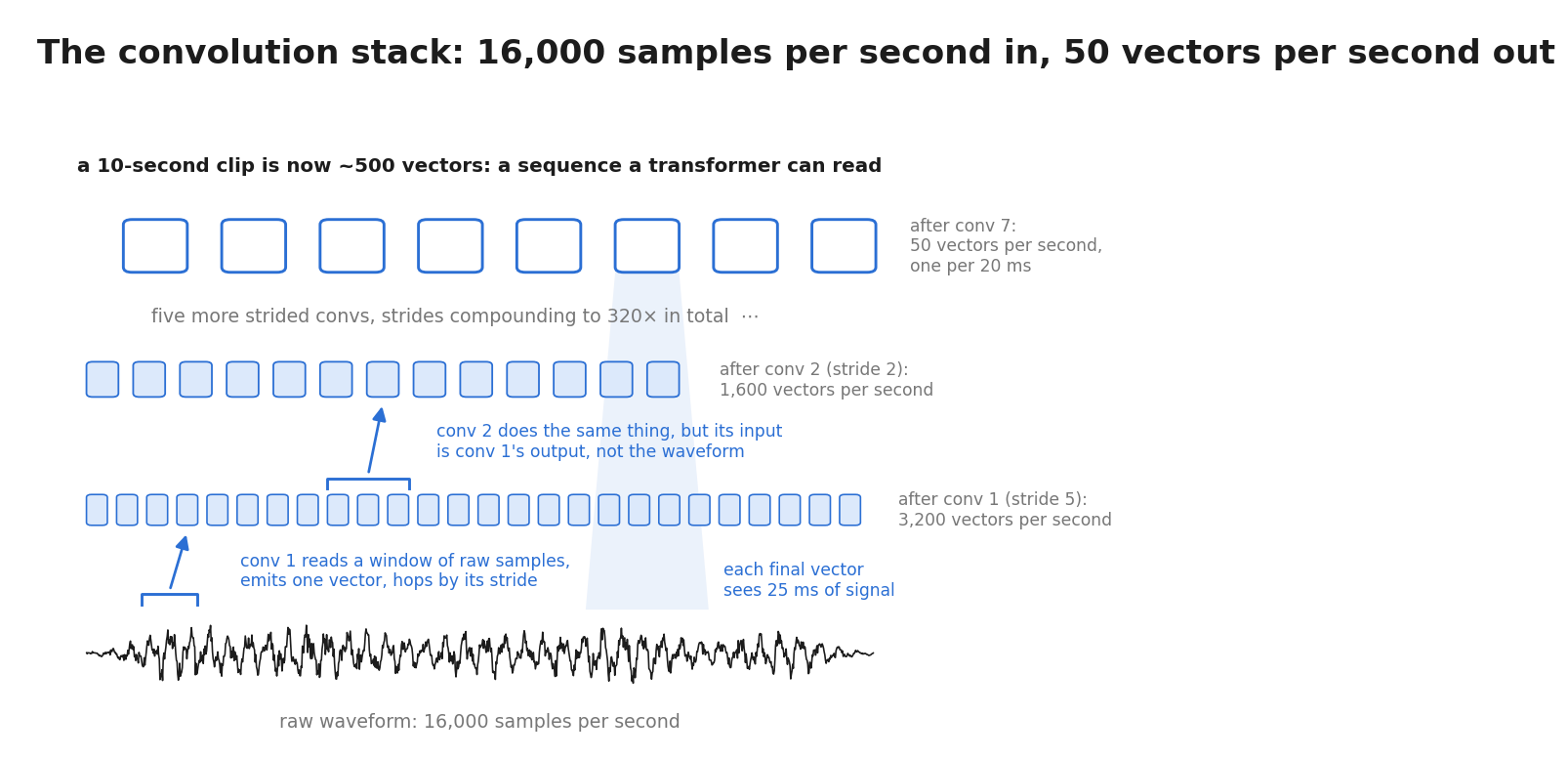
Fig. 1: The convolution stack that turns a waveform into frame vectors. Conv 1 slides its window over raw samples; conv 2 slides its window over conv 1's output, not the waveform; and each layer's stride shrinks the sequence again. Seven layers compound to 320×: 16,000 samples per second become 50 vectors per second, each covering 25 ms of signal.

Option 2: use a hundred years of signal processing (AST, AudioMAE, BEATs). The building block is the Fourier transform. It rests on one mathematical fact: any stretch of signal, however messy, can be rewritten as a sum of sine waves of different frequencies, and the transform computes how much of each frequency that sum contains. A frequency band is just a range of those frequencies: 0 to 100 Hz, 100 to 200 Hz, and so on up to 8,000 Hz (the highest frequency a 16 kHz recording can represent). The number recorded for each band is the energy: how strongly the signal oscillates at those rates within the window.

So: apply the transform to a 25 ms window of waveform (400 samples) and you get a list of energies, one per band, a single column of numbers summarizing that slice of the signal. Concretely, a voice speaking at a 120 Hz pitch puts large numbers in the bands around 120 Hz; wind puts moderate numbers across the lowest bands; hiss puts small numbers across the high ones.

Now slide. The window is 25 ms wide but moves forward only 10 ms per step, so consecutive windows overlap by 15 ms and you get 100 columns per second. Stack the columns side by side and you have a 2-D array: time on one axis, frequency on the other, energy as brightness. One last adjustment: human ears resolve low frequencies much more finely than high ones, so warp the frequency axis onto a matching log-like scale (the mel scale) and keep 80 bins. The result is a mel-spectrogram: for our ten-second clip, roughly 1,000 time steps by 80 frequency bins.

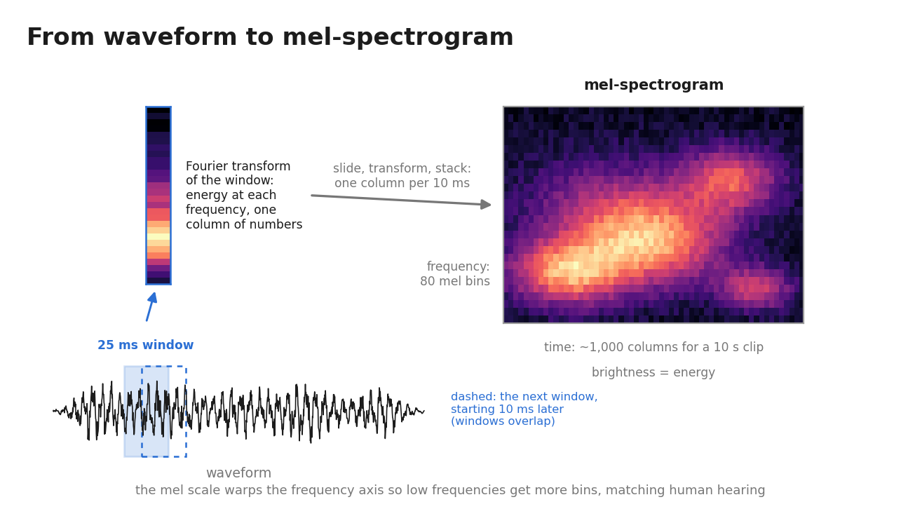
Fig. 2: From waveform to mel-spectrogram. Each 25 ms window becomes one column of energies via the Fourier transform; slide the window in 10 ms hops and the columns stack into a 2-D array with time on one axis, frequency on the other, and energy as brightness.

Look at what we just did: we turned sound into an image, and different sounds look visibly different in it. A voice draws horizontal bright bands (its pitch and the frequencies it emphasizes, held over time), a short bark is a brief vertical stripe (energy at many frequencies at once, for a moment), and steady wind fills the low-frequency rows. And once your audio is an image, computer vision methods apply directly: cut it into patches and run a ViT (Vision Transformer) over them. That is exactly what AST, AudioMAE, and BEATs do.

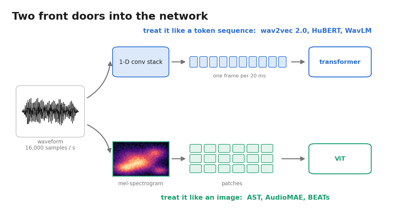
Fig. 3: The two input pipelines. Option 1: learn filters with 1-D convolutions and treat audio like a token sequence. Option 2: compute a mel-spectrogram and treat it like an image.

Neither option is more correct. Speech is structured like text: a language uses only a few dozen distinct sounds (phonemes), produced one after another, with rules about which can follow which, the same way text is a sequence of words drawn from a vocabulary. That is the kind of data BERT-style methods were built for. Ambient sound is structured like an image texture, energy patterns spread over time and frequency, which is the kind of data vision-style methods were built for. A real recording usually contains both at once (a sentence and the wind, in one waveform), so neither view can be dismissed, and the field kept both approaches. Knowing which input representation a model uses tells you a lot about it immediately.

We can now get audio into a network. What do we want out of it?

3. What we actually want: a vector where distance means something

For most practical purposes, what you want from an audio model is an embedding: one vector, maybe 768 floats, summarizing a clip, with the property that distances in the vector space are meaningful: the embeddings of similar clips should sit close together, and the embeddings of different clips far apart. Get that and a pile of hard problems reduce to distance computations:

• Search: embed your library, embed the query, return nearest neighbors.
• Classification: keep the encoder frozen, and train just a small linear layer on top of its embeddings.
• Speaker verification: "is this the same voice?" becomes a cosine similarity against a threshold.
• Recommendation, deduplication, clustering: each reduces to comparing distances between embeddings.
• Multimodal LLMs (large language models): every model that "hears" is an audio embedding model bolted onto a language model.

Note the mismatch with §2, though: the encoders there produce a vector per frame, while everything on this list wants one vector per clip. The clip vector only exists if you make one, usually by averaging the frame vectors. Some training objectives score the frames, some score the clip summary, and this distinction will matter later.

Everything so far is engineering. The real problem is conceptual: I said the embeddings of similar clips should sit close together. Similar how? Take a concrete five-second recording: a woman says "the tide is coming in" on a windy beach, and a dog barks in the background. What should be near it?

• The same sentence read by a stranger in a studio? (Same words.)
• The same woman saying something else? (Same voice.)
• The same beach with nobody talking? (Same scene.)
• A different dog in a park? (Same event.)

Every answer is defensible, and they point in completely different directions. The reason the question has no single answer is a fact about the signal itself: the words, the voice, the scene, and the events are all present simultaneously, superimposed in one waveform. Any definition of "similar" privileges one of these layers, and a model that pulls two clips together along one layer must, to some degree, ignore the others.

So "similar" is not a property of audio. It's a choice. And you never get to make the choice directly. There is no principled "embedding loss" you write down that says "please arrange clips by meaning." What actually happens, in every model in this post, is this: you train the network on some task, and the embedding is the residue, the internal arrangement of inputs the network was forced into in order to do the task. Pick the task and you've picked which layers of the signal survive into the vector and which get erased. A network trained to transcribe keeps the words and forgets the voice. A network trained to detect barks keeps the events and forgets the words.

The rest of this post is the history of that choice: the tasks people trained on, what each task's residue kept and destroyed, and how the field moved toward embeddings that keep more. The history ran in three phases: supervised labels first (§4), then self-supervision with no labels at all (§5), and language supervision last (§6).

4. The obvious thing first: supervised classification

Through the 2010s the standard approach was: collect labels, train a classifier with cross-entropy, and use the trained network's penultimate layer as the embedding. The mechanism: to classify well, the network must arrange inputs in its last hidden layer so that a linear boundary can separate the classes, and any arrangement good enough for that turns out to transfer to other tasks.

Recall from §3 that one clip carries several layers of information at once: the events, the voice, the words. Under supervised training, each of these got its own labels and its own models:

Signal layer	Training task	Models	Where the embedding comes from
Events	Tag a clip with the sounds it contains. Dataset: AudioSet (Google, 2017), 2 million YouTube clips labeled with 527 classes ("dog bark", "siren", "acoustic guitar").	VGGish (a CNN, trained on a YouTube precursor of AudioSet), then PANNs (larger CNNs), then AST (Audio Spectrogram Transformer)	The penultimate layer, reused as a general-purpose sound-event embedding.
Voice	Classify "which of these 7,000 speakers is talking?"	x-vectors (2018)	The penultimate layer. To tell speakers apart it must place clips of the same person close together regardless of what is being said: a voice embedding.
Words	Transcribe audio into text (ASR, automatic speech recognition).	Deep Speech 2 (Baidu, 2015), Listen, Attend and Spell (Google, 2015)	The late layers, one vector per frame rather than per clip, since the output is a character sequence and not a single class. A network cannot transcribe a clip without internally representing its words.

This approach works, but it has two problems. First, the label list is a ceiling: a 527-way classifier is only ever asked one question per clip, and the objective actively rewards discarding everything the labels don't mention, because invariance to it makes classification easier. The event model discards the words and the voice; the speaker model discards the words and the scene. One clip, four layers, and every label list picks one and discards the rest.

Second, labels are expensive, and in audio more than anywhere. AudioSet took a Google team years and is still noisy. Transcription is worse: an hour of speech costs many hours of human labeling, and most of the world's languages have essentially no transcribed audio at all. Meanwhile unlabeled audio (podcasts, radio, videos, voice notes) is functionally infinite.

Here's where audio's history forks from vision's. When vision hit its label ceiling, it found billions of images with free text attached (alt-text) and trained on that text instead of labels: that's CLIP (Contrastive Language-Image Pretraining), 2021. Audio had no equivalent; the internet does not caption sound at scale. Speech research had unlimited unlabeled audio and could not afford labels, so it did what only became standard elsewhere years later: drop the labels entirely and make the audio teach itself.

5. Let the audio teach itself

5.1 The idea, and the trap

How can data with no labels teach anything? The answer is the same idea BERT uses for text: hide part of the input and predict it from the rest.

Mask out a few hundred milliseconds from the middle of our beach clip and ask the model to predict the missing frames. Predicting them well requires encoding several things at once. The missing frames contain the woman's voice, so the model must encode how her voice sounds. The wind continues across the masked region, so the model must encode the background sound. The sentence so far is "the tide is...", so predicting the rest requires phonetics and vocabulary: "coming" is far more likely than "purple". None of this needed a label. It did not even need a name: there is no word for the exact sound of this wind or this voice, but the prediction task forces the model to represent them anyway. The residue of this task could be an embedding that keeps every layer of the signal at once.

But the naive implementation fails. The obvious setup is: run the encoder on the masked clip, and take its output at each masked position as the prediction; run the same encoder on the audio that was masked out, and take its output as the target; make the loss the distance between prediction and target. To see the failure, ask what the cheapest way to drive this loss to zero is. The loss only rewards making the prediction match the target; nothing rewards distinguishing one clip from another. So the cheapest solution is to ignore the input and always output the same constant vector. Prediction equals target for every frame of every clip, the loss is zero, and the model has learned nothing.

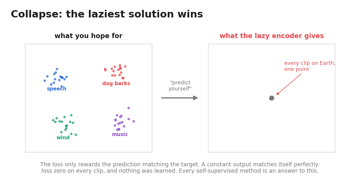
Fig. 4: Collapse. Nothing in "predict yourself" rewards distinguishing clips, so the constant output wins and every clip maps to the same point.

This is called collapse, and it's not a bug in one paper; it is inherent to any setup where a model grades itself against itself. Supervised training never had this problem: the labels differ across inputs, so a constant output scores terribly. The moment the targets come from the model itself, the constant solution becomes available. Every landmark self-supervised audio model is a different way of blocking it, and the easiest way to organize them is by a single question: what exactly should the model predict at the masked position?

5.2 Answer 1: the true frame, picked out of a lineup (wav2vec 2.0)

First answer: don't reproduce the missing frame, recognize it. Show the model the true frame plus a set of impostors and train it to pick out the right one. Now the constant solution is worthless: a constant scores every candidate equally. This is contrastive learning. It came to speech through three models, each fixing a weakness of the previous one:

• CPC (Contrastive Predictive Coding, 2018) introduced the setup. Encode the clip into a sequence of frame vectors. Given the frames up to some point, train the model to pick the true next frame out of a small set that also contains frames taken from other positions and other clips. The method is not audio-specific: the paper ran it on speech, images, and text.
• wav2vec (Meta, 2019) applied CPC to raw speech waveforms and showed that it pays off: pretrain this way on unlabeled speech, then train a speech recognizer on the resulting frame vectors, and the error rate drops. But it had two limits. First, it predicts the future from the past, so the audio after a position is never used as context. Second, its frame vectors are continuous, while BERT-style training predicts discrete tokens. The follow-up vq-wav2vec addressed the second limit with a quantization step. Keep a small table of vectors called a codebook; its entries start random and are trained along with the rest of the network. Replace each frame vector with the codebook entry nearest to it. Every frame is now one of a fixed set of entries, so the audio becomes a sequence of discrete units that can be treated like text tokens.
• wav2vec 2.0 (Meta, 2020) combined the pieces into a single model and removed the first limit: instead of predicting the future from the past, mask spans in the middle of the clip and predict them using context from both sides, exactly like BERT. This is the version the rest of the field built on, and the one worth understanding in detail.

Concretely:

1. The 1-D convolution stack from §2 turns the waveform into frame vectors $z_t$, one per 20 ms.
2. Spans of frames get masked; a transformer reads the corrupted sequence and outputs a context vector $c_t$ at each position.
3. Each true frame vector gets quantized: replaced with the nearest entry of a learned codebook, the vq-wav2vec mechanism from above. This gives a discrete target $q_t$. Quantizing keeps the lineup well defined: the candidates are distinct codebook entries rather than continuous vectors that can sit arbitrarily close to each other.
4. At each masked position, the model is given $q_t$ plus 100 impostors (quantized frame vectors from other masked positions in the same clip) and must identify the true one.

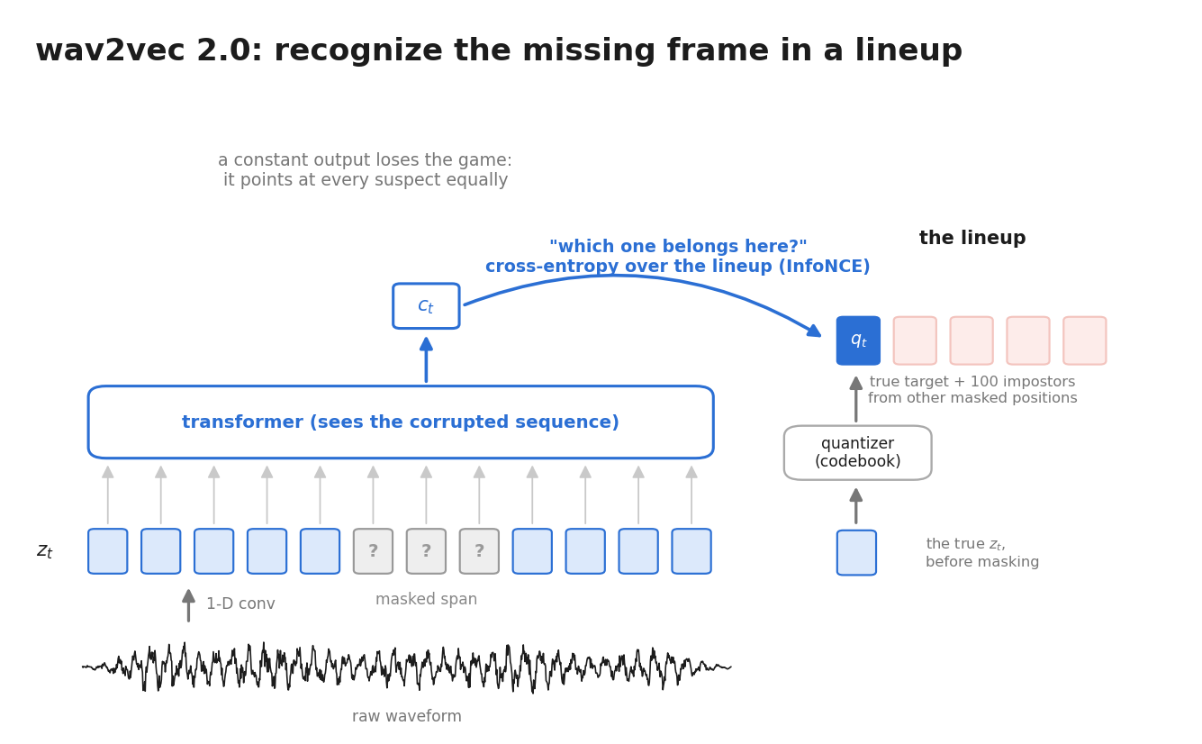
Fig. 5: One wav2vec 2.0 training step at one masked position: the context vector $c_t$ must pick the true quantized frame $q_t$ out of a lineup of impostors from the same clip.

"Pick the right one out of K" is a classification problem, so the loss is cross-entropy, the same loss used in supervised classification. As a reminder of how it works: a classifier ends with one raw score per candidate (the logits); softmax turns the scores into probabilities; cross-entropy is minus the log of the probability assigned to the correct candidate, near zero when the model is confidently right and large when it is confidently wrong. Here the logits are similarities between $c_t$ and each candidate:

$$\mathcal{L}_t = -\log \frac{\exp(\mathrm{sim}(c_t, q_t)/\kappa)}{\sum_{\tilde{q} \in Q_t} \exp(\mathrm{sim}(c_t, \tilde{q})/\kappa)}$$

where $Q_t$ is the lineup, $\mathrm{sim}$ is cosine similarity, and $\kappa$ is a temperature (cosines live in $[-1, 1]$, too flat a range for a softmax to bite on, so we stretch them). The literature calls this loss InfoNCE: cross-entropy where the classes are the members of the lineup, assembled fresh at each masked position instead of fixed in advance.

Two caveats:

1. The codebook can collapse too. Nothing forces the network to use all of the codebook entries, and the prediction task gets easier if it uses fewer: if every frame snaps to the same entry, the target and the impostors become identical vectors, and the lineup can be won without learning anything. wav2vec 2.0 adds a diversity penalty, an extra loss term that rewards using all codebook entries at similar rates across a batch.
2. The impostors come from the same clip as the target. That includes frames that contain the same sound, for example the "s" in one word and the "s" in another word. The loss pushes their representations apart even though they sound alike, so the objective that prevents collapse also erases some genuine similarity.

The headline result from the paper: pretrain on 60,000 hours of unlabeled speech, then fine-tune on ten minutes of transcribed audio, and the model reaches a 4.8% word error rate on the clean LibriSpeech test set. Ten minutes of labels is enough because pretraining had already forced the representations to encode the phonetic structure that transcription needs.

5.3 Answer 2: cluster tags, fixed before training (HuBERT, WavLM)

The second answer changes what the classes are. In wav2vec 2.0 the candidate set was rebuilt at every masked position: the true frame plus impostors sampled on the spot. The second answer instead uses one fixed list of classes shared by every frame in the corpus, like BERT's token vocabulary. That requires a class label for every frame, and no such labels exist. HuBERT (Hidden-unit BERT, Meta 2021) manufactures them: before training starts, it assigns every frame a pseudo-label, built from simple handcrafted audio features:

1. Compute MFCCs (Mel-Frequency Cepstral Coefficients), a handcrafted 1970s-era summary of each frame's spectrum, for every frame of the corpus.
2. Run k-means with 100 clusters over them. Now every frame in the corpus carries a cluster ID, 0 to 99. These tags are bad. MFCC clusters mean little beyond "sounds vaguely alike."
3. Train exactly like BERT: mask spans, predict each masked frame's tag, plain cross-entropy over 100 classes.
4. After this first round of training, the model's internal features describe the audio far better than MFCCs do. The paper scores cluster quality by how well cluster IDs align with ground-truth phoneme labels (phone purity and mutual information), and clusters built from the model's middle-layer features score far higher than MFCC clusters. So re-cluster the corpus using the model's own middle-layer features (500 clusters this time), replace the old pseudo-labels with the new cluster IDs, and train again.

labels = kmeans(mfcc(corpus), k=100)                # crude tags, fixed before training
for iteration in range(2):
    model = train_bert_style(corpus, labels,        # mask spans; cross-entropy on the
                             loss_on=masked_only)   #   cluster ID of each masked frame
    labels = kmeans(model.layer_features(corpus),   # re-tag the corpus with the model's
                    k=500)                          #   own, much better features

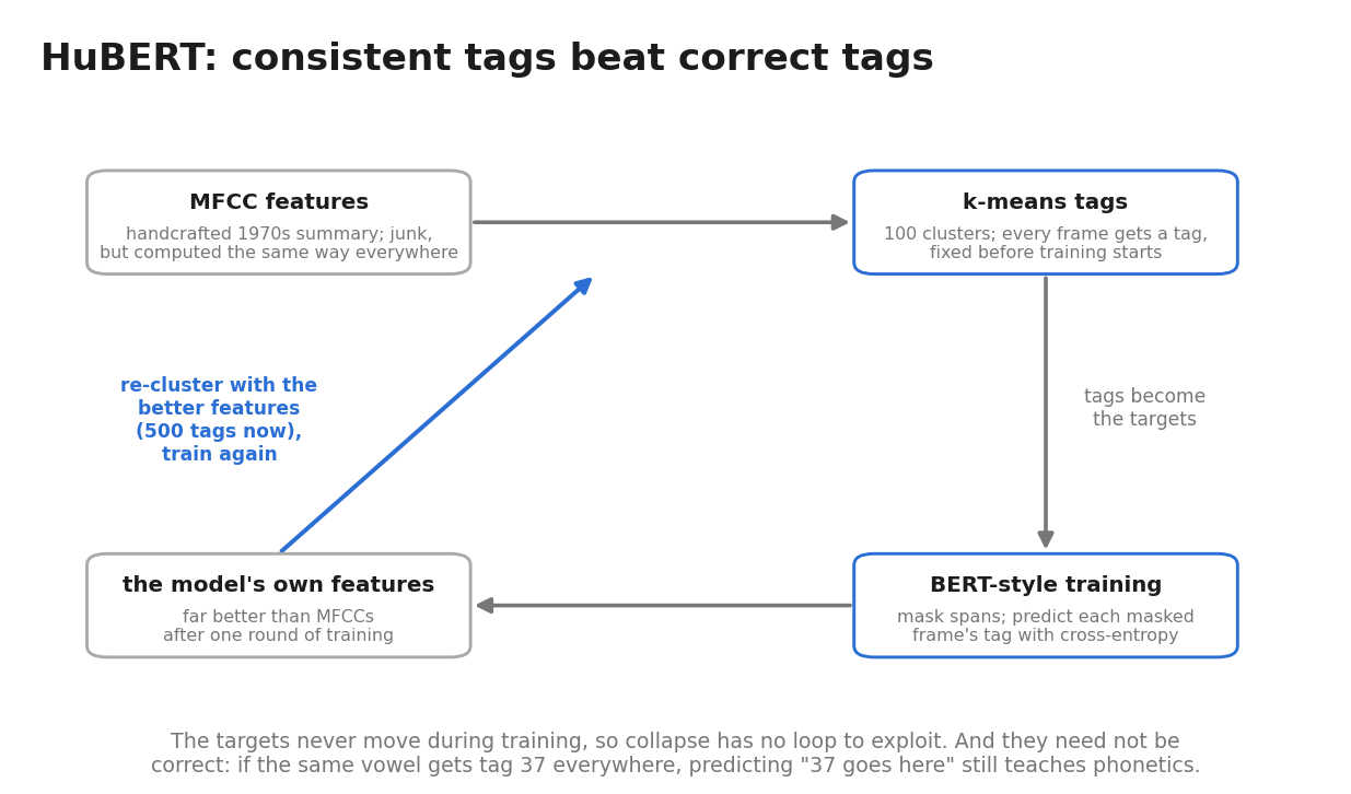
Fig. 6: The HuBERT bootstrap. Crude features get clustered into tags, the tags supervise masked prediction, and the model's much better features get re-clustered into the next round's tags.

Collapse is not possible here: the targets are computed offline and never move during training, so the model has no way to influence them. The real question is why bad tags teach anything at all: targets don't need to be correct, they need to be consistent. If the same vowel sound gets tag 37 everywhere it occurs, then learning to predict "37 goes here" from context forces the model to learn everything that predicts that vowel: the phonetic environment, the speaker's habits, the acoustics of the room. Whether tag 37 "means" anything is irrelevant.

A historical aside. Vision tried clustering-as-supervision too (DeepCluster, SwAV), and there it stayed a side branch; vision's crown went to self-distillation (BYOL, DINO). In speech, clustering won: HuBERT became the field's backbone. Why the reversal? Most likely because speech, unlike photographs, really is built from a small discrete inventory (phonemes, a few dozen per language), so cluster IDs match the data's true shape, and there is no analogous finite alphabet of image patches. When a method's structure matches the signal's structure, it sticks.

WavLM (Microsoft, 2021) is HuBERT with one change to the input. The training objective is identical: mask spans, predict each masked frame's cluster tag. But during training the input gets corrupted: a second speaker, or noise, is overlaid on part of the clip, while the targets stay the ones computed from the clean original. To predict the clean tags through the interference, the model has to track which speaker is the main one, not just what is being said. In §3's terms: pure content prediction was slowly erasing the voice layer, and this change forced the model to keep it. WavLM ranked first on the SUPERB leaderboard (Speech processing Universal PERformance Benchmark), which evaluates one frozen encoder on a dozen tasks (recognition, speaker ID, emotion, and diarization, which means splitting a recording by who speaks when), because its embedding keeps more layers of the signal than encoders trained on clean input alone.

One unplanned side effect worth knowing: HuBERT's tags are discrete, so you can treat them as tokens and train a language model directly on speech, with no text anywhere in the pipeline. That's "textless NLP" (GSLM, Generative Spoken Language Modeling), and it seeded today's speech-native LLMs.

5.4 Answer 3: an EMA teacher (data2vec)

The third answer is the self-distillation idea from vision (BYOL, DINO). Keep two copies of the network, identical at initialization. The student trains normally. The teacher is never trained by gradients: after each step its weights just drift a small fraction toward the student's, making it an exponential moving average (EMA) of the student's own past. The student receives the masked clip; the teacher receives the unmasked clip. At each masked position, the student is trained to predict the feature vector the teacher produced there, with a plain regression loss: match the teacher's vector directly.

Why doesn't this collapse? Because gradients flow only through the student; the teacher's weights receive none. Collapse required the optimizer to move the targets toward a constant, and here the targets come from the teacher, which the optimizer cannot touch. This closes the direct route to collapse, but not every route: the teacher's weights follow the student's through the EMA update, so a student drifting toward constant outputs would slowly pull the teacher's targets along with it. That remaining pressure is why data2vec also normalizes its targets, as described below.

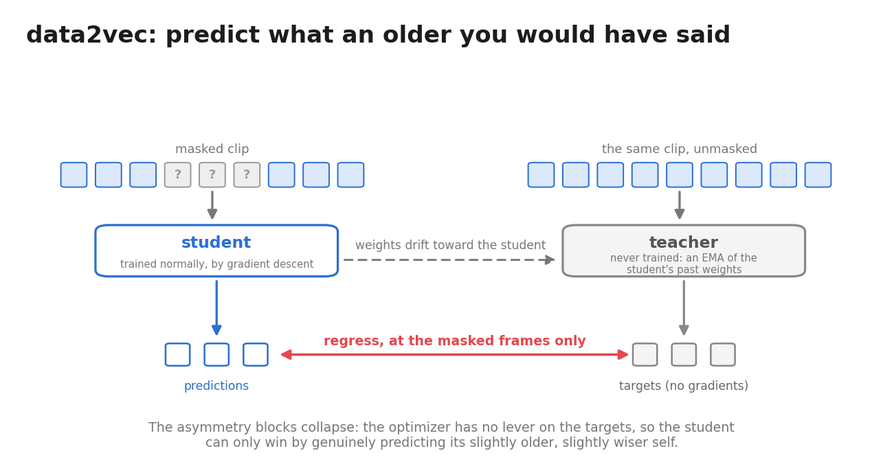
Fig. 7: data2vec. Student sees the masked clip, teacher sees the whole clip, and the student regresses the teacher's features at the masked frames. The teacher only ever drifts toward the student.

In audio this is data2vec (Meta, 2022). The paper's central claim is that the method is modality-independent: the identical scheme trains speech, image, and text encoders, and on speech it matches or beats wav2vec 2.0 and HuBERT. Two implementation details carry weight. First, the targets are an average of the teacher's top several transformer layers, not just its final one. Second, the targets are normalized, so their variance cannot shrink toward zero during training; this blocks the slow route to collapse described above. In practice HuBERT and WavLM remained the more widely used speech encoders, but data2vec demonstrated that one masked-prediction scheme can serve every modality.

5.5 Answer 4: frozen random targets (BEST-RQ)

HuBERT showed the targets only need to be consistent. BEST-RQ (BERT-based Speech pre-Training with Random-projection Quantizer, Google 2022) asks the obvious follow-up: if the targets only need to be consistent, why learn the targets at all? Its targets are built in three steps:

1. Take each frame's mel-spectrogram vector (the Option 2 features from §2).
2. Multiply it by a random matrix that is fixed at initialization and never trained.
3. Find the nearest entry in a codebook of random vectors, also fixed and never trained. The index of that entry is the frame's tag.

Steps 2 and 3 do the same job k-means did for HuBERT: partition the feature space into regions and give every frame the ID of the region it lands in. The difference is where the region boundaries come from. k-means fits them to the data, and HuBERT re-fits them each iteration with better features; BEST-RQ draws them at random once and never moves them. Training is then identical to HuBERT: mask spans, predict each masked frame's tag with cross-entropy. No k-means, no iterations, no learning anywhere in the target path.

Random targets have every property the previous sections showed matters. They cannot collapse: they are fixed before training and never move. The model cannot make them easier: nothing in the target path is trainable. And they are consistent: the projection and the codebook are deterministic, so the same input features get the same tag every time. The approach also scales: BEST-RQ is the pretraining behind Google's USM (Universal Speech Model) family, trained on millions of hours of speech.

Now line up the four answers. wav2vec 2.0's targets were a codebook trained jointly with the model. HuBERT's were clustered offline from crude features. data2vec's were a moving average of the past. BEST-RQ's are frozen random noise. The targets got simpler at every step, and the models kept getting better. For masked prediction, the intelligence belongs in the model, not in the targets; the target's only job is to be consistent and out of the model's control.

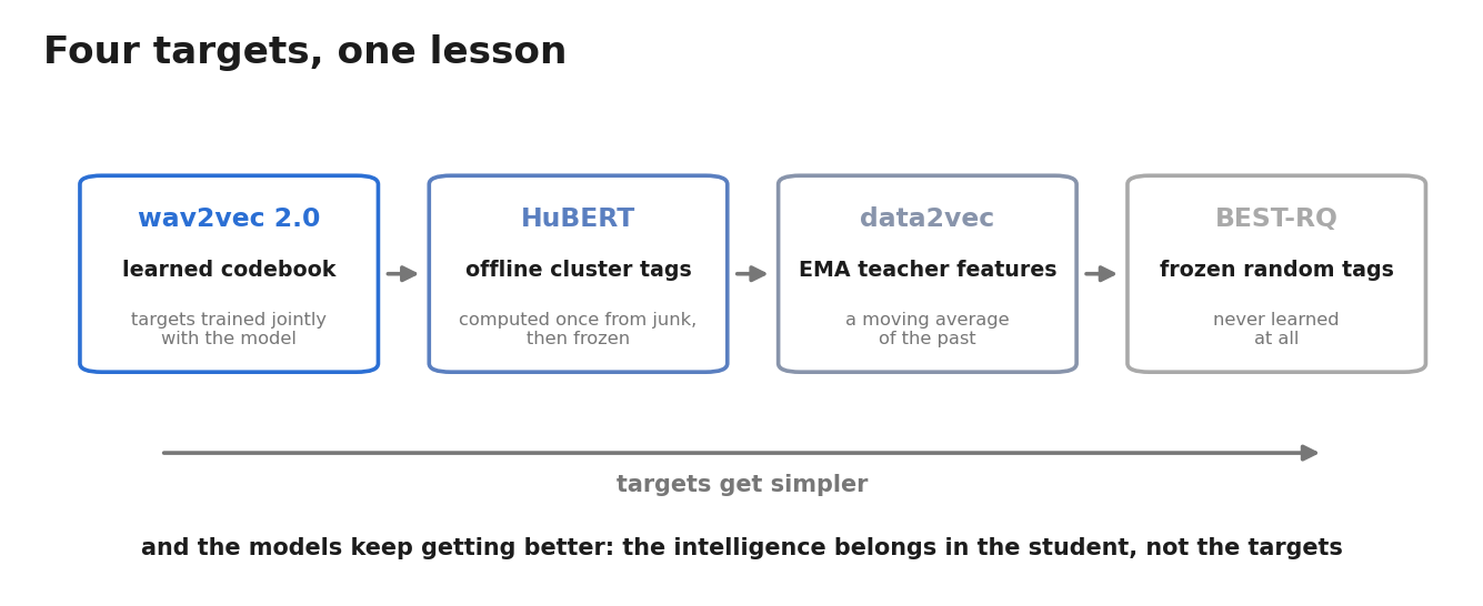
Fig. 8: The arc of the target. Each generation asked less of the target and more of the model, and quality kept going up.

5.6 The same ideas on spectrograms (AudioMAE, BEATs)

Every model in §5 so far reads the raw waveform, chopped into frame vectors by a convolution stack (Option 1 from §2). The same self-supervised ideas also work on the other input representation, the mel-spectrogram (Option 2), cut into patches and treated the way vision models treat an image.

AudioMAE (Meta, 2022) applies masked autoencoding to the spectrogram: mask 80% of the patches and train the model to reconstruct the missing values. The reconstruction runs through a small decoder that is discarded after training; only the encoder is kept. Collapse is not a concern here, because the targets are the input values themselves, which the model cannot change.

BEATs (Bidirectional Encoder representation from Audio Transformers, Microsoft 2022) runs HuBERT's recipe on spectrogram patches: convert each patch to a discrete token, mask patches, and predict the tokens at the masked positions. The first tokenizer is random, as in BEST-RQ. Training then alternates, the same bootstrap as HuBERT's re-clustering: the trained model is used to build a better tokenizer, and the better tokenizer's tokens train a better model. BEATs set the state of the art on AudioSet tagging without using any labels during pretraining, and its encoder is now one of the standard audio encoders attached to audio LLMs.

At this point you can read any new audio self-supervision paper and place it in about a paragraph: which input representation does it use, and what does it predict at the mask?

5.7 One more family: declared similarity (TRILL, COLA, BYOL-A)

One more self-supervised family remains. It is minor in audio, but it shows §3's point, that "similar" is a choice, more directly than any other method. Instead of masking, these methods declare two things similar and train the encoder to place them close together:

• TRILL (Google, 2020) declares two segments cut from the same recording, a few seconds apart, to be similar. Consider what that choice keeps. Across a few seconds of gap, the voice, the recording conditions, and the speaking style stay the same; the words change. So the embedding keeps the stable properties and discards the words. TRILL was built for exactly that: speaker, emotion, and health signals, the complement of a transcription model.
• COLA (2020) makes the same declaration as TRILL (two segments of the same recording are similar), but trains with the InfoNCE loss from §5.2: the lineup for a segment contains its partner segment as the true answer and segments from other clips in the batch as impostors.
• BYOL-A (2021) declares two augmented versions of the same segment similar: mix in background noise, warp the spectrum. The two versions are matched through an EMA teacher, the same mechanism as §5.4, so no impostors are needed.

In all three, the definition of "the same" determines which layers of the signal the embedding keeps.

6. Language finally shows up

By around 2021, audio had strong label-free encoders. What it did not have was a connection to language: a HuBERT embedding cannot be searched with a text query, and its dimensions have no names. Vision solved this with CLIP. The audio equivalent arrived late, because, as §4 noted, the internet has no large supply of text paired with audio. And it arrived split in two, because text about audio comes in two kinds. A transcript records what was said. A description records what it sounded like. Training on one or the other produces different models with different residues.

6.1 Whisper: supervise on transcripts, keep the words

For speech specifically, the internet does have text at scale: subtitles, captioned videos, audiobooks read from known books. Whisper (OpenAI, 2022) trains on it at scale: 680,000 hours of web audio paired with transcripts, an encoder-decoder transformer trained to generate the transcript token by token (plus language tags, timestamps, translations, all signaled by special tokens).

Whisper is a speech recognizer; it was never trained to produce embeddings. But §3's argument applies here too: the embedding is the residue of the training task. The decoder can only emit a word if the evidence for that word exists in the encoder's frame features, and it must emit every word. So the encoder's features are forced to carry essentially everything linguistic, and that residue turned out to be the strongest word-layer representation in the field. Today Whisper's encoder is the default speech encoder attached to multimodal LLMs (Qwen2-Audio among many).

The cost is the same trade §4 described. What transcription does not need, the features do not keep: speaker identity, the recording conditions, the emotion. These are preserved only to the extent that they help predict the next transcript token, and they rarely do. Whisper's embedding carries little information about who is speaking.

6.2 CLAP: supervise on descriptions, keep the events

For everything that isn't speech, there are no transcripts, only descriptions: "a dog barks while wind blows into the microphone." CLAP (Contrastive Language-Audio Pretraining, Microsoft 2022; the widely used open build is LAION-CLAP) collects (clip, caption) pairs and trains two encoders, an audio tower (a spectrogram encoder, pooled to one clip vector) and a text tower, to land matching pairs close together in one shared space.

The loss is the InfoNCE lineup from §5.2, with different candidates. For each clip in a batch of $N$ pairs, the lineup is the $N$ captions in the batch; the clip's own caption is the correct answer, and cross-entropy scores the choice. The same loss runs symmetrically in the other direction: each caption must pick its clip out of the $N$ clips. The important change is what the candidates are. In §5.2 they were frames. Here the candidates are sentences, drawn fresh every batch. The label vocabulary is no longer a fixed list of 527 tags; it is language.

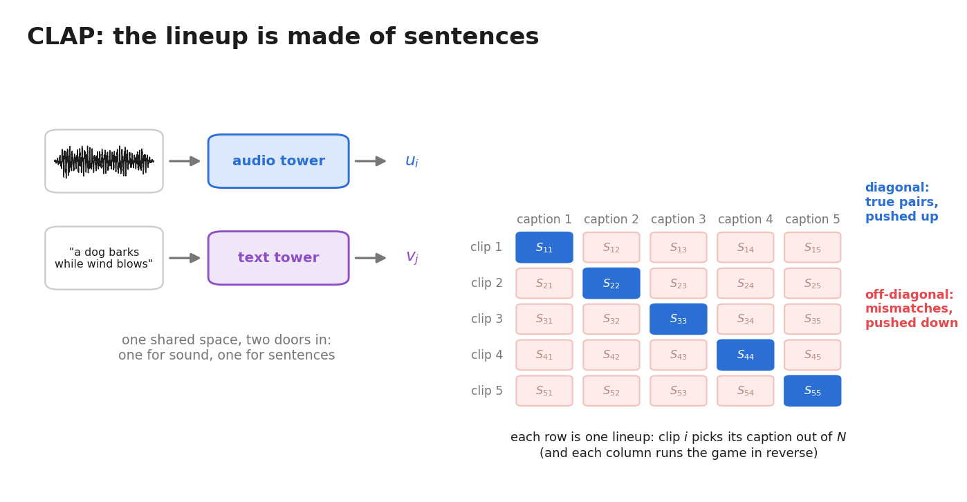
Fig. 9: CLAP's training signal. Two towers, one shared space, and an $N \times N$ similarity matrix per batch: diagonal (true pairs) pushed up, everything else pushed down. Each row is a lineup whose candidates are sentences.

A shared audio-text space enables zero-shot classification, the capability CLIP made famous: embed the sentences "a dog barking" and "a cat meowing," embed the clip, and assign the label whose sentence is closer. This is a classifier built from prose, for any label set, with zero training examples. LAION-CLAP reaches 90% zero-shot accuracy on ESC-50, a standard environmental-sound benchmark. Text-to-audio search works the same way: embed the query sentence, and ranking clips is a dot product. Sound-effect libraries use this today.

So why did CLAP not have the impact CLIP had? Two reasons. First, the data is small. CLIP trained on 400 million image-text pairs collected from alt-text. Audio caption datasets are hand-assembled and three to four orders of magnitude smaller: LAION-Audio-630K is 630 thousand pairs. Second, captions describe events. People write "a dog barks." They do not write down the sentence being spoken, and they never describe the voice. So CLAP's residue is an event-layer embedding that can be queried with text: our beach clip embeds as speech-plus-dog-plus-wind, and the words and the voice are lost.

Put §6.1 and §6.2 side by side: Whisper keeps only the words, and CLAP keeps everything except the words. Both also lose whatever text never records at all: the specific sound of the wind, the reverb of the room, the qualities that make a voice recognizable. The §5 models capture all of that, but they cannot be queried with text. So no single model both keeps every layer and connects to language; §8 returns to this gap.

7. Turning many frames into one clip vector

The masked-prediction objectives of §5 score predictions at individual frames, so their native output is a sequence of frame vectors. That suits tasks that consume sequences, like recognition and diarization. But nothing in those objectives ever produced or evaluated a single whole-clip vector, and search, deduplication, and clustering all need one vector per clip. There are three ways to get one:

1. Pool. Average the frame vectors, or let a small attention head weight them before averaging (attentive statistics pooling). Simple, and it works. One practical fact matters here: the layers of a speech transformer specialize. Probing studies (Pasad et al., and SUPERB's per-task learned layer weights) consistently find speaker identity concentrated in the early layers, phonetic content peaking near the middle, and word-level information peaking about two-thirds of the way up, with both content measures falling again in the topmost layers of a pretrained model. A frozen HuBERT contains both the voice information and the word information, stacked at different depths, so choosing which depth to pool from is choosing which layer of the signal the clip vector keeps. The superposition from §3 did not go away; it moved inside the network.

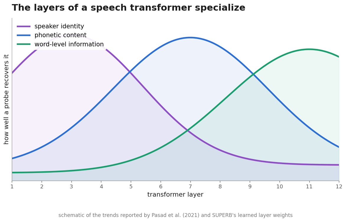
Fig. 10: Where the layers live inside a self-supervised speech model, schematically (after Pasad et al., 2021). Speaker identity is strongest early; phonetic content peaks near the middle; word-level information peaks about two-thirds of the way up. In a pretrained model both content curves then fall in the final layers, whose representations drift back toward the input (fine-tuning removes this drop). Probe a different depth, extract a different layer of the signal.

2. Train the clip vector directly. Some objectives already produce one vector per clip. CLAP pools its audio tower's frame vectors into a single clip vector before the loss, so the caption-matching loss trains that vector itself. The §5.7 methods work the same way: each declared-similar pair is compared as two pooled vectors. In these models the clip vector is what training optimizes, not something derived afterwards.

3. When the similarity has a definition, train on the definition. Suppose the layer you want is the voice: the question is "are these two clips the same speaker?", as in verification and diarization. Unlike §3's question, where "similar" had many defensible answers, this one has a ground truth: two clips either are or are not from the same speaker. So train on it directly: pull same-speaker clips together, push different-speaker clips apart. This is called metric learning. The standard model is ECAPA-TDNN, trained on thousands of labeled speakers with an additive angular margin softmax (AAM-softmax): each speaker's utterances are forced into a tight cone of directions, and the cones of different speakers must be separated by a margin. This is the same loss (ArcFace) used in face recognition, for the same reason: at test time the speakers are people the model has never seen, so it cannot rely on its training classes; it needs an embedding where distance alone decides "same or different," and the margin between cones is what makes distance reliable on new speakers. These embeddings run production speaker-verification systems. Self-supervised features come close in probes (WavLM especially), but when you know exactly what you mean by "similar," training on that definition beats hoping it emerges from another task.

8. Putting it all together

Everything in this post, in historical order:

2010s   supervised classifiers          one layer per label list
        ├─ AudioSet -> VGGish/PANNs/AST      the events
        ├─ speaker IDs -> x-vectors          the voice
        └─ transcribed ASR                   the words
                 │
                 │   labels too expensive; each list erases the other layers
                 ▼
2018+   the self-supervised turn        "predict the hidden part of yourself"
        ├─ CPC -> wav2vec 2.0    target = true frame in a lineup      (negatives)
        ├─ HuBERT -> WavLM       target = offline cluster tag         (consistency > correctness;
        │                                                              WavLM re-learns the voice)
        ├─ data2vec              target = EMA teacher's features      (asymmetry)
        ├─ BEST-RQ               target = frozen random tag           (intelligence in the model)
        ├─ AudioMAE / BEATs      masked prediction on spectrogram patches
        └─ TRILL / COLA / BYOL-A "similar" is declared directly
                 │
                 ▼
2022+   language arrives late
        ├─ Whisper               generate the transcript              (all words, no voice)
        └─ CLAP                  match clip to caption                (all events, no words)

Two questions place every model. One: who defines "similar", the signal itself, human labels, or language? Two: which layer of the signal does the embedding keep: words, voice, events, music, or everything, entangled?

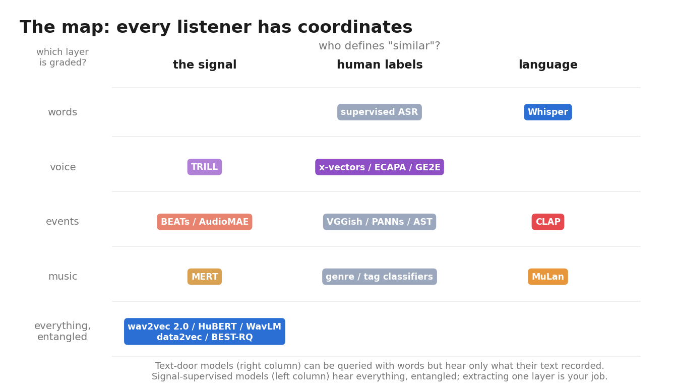
Fig. 11: Every encoder in one grid. Columns: who defines "similar". Rows: which layer of the signal the embedding keeps. Each model in this post is one cell.

Answer both questions and the practical guide writes itself:

Task	Encoder	Why
Zero-shot sound tagging; text-to-audio search	CLAP (the LAION-CLAP build)	Its text and audio embeddings share one space, so a text query ranks clips directly
Speech recognition; searching what was said	Whisper's encoder; or wav2vec 2.0 / HuBERT / WavLM with a small decoder on top	Their features carry the word layer
Speaker verification, diarization, voice similarity	ECAPA-TDNN; or WavLM with a probe on its early layers	Trained (or probed) specifically for the voice layer
Sound-event tagging with a frozen encoder	BEATs or AudioMAE	Event features learned without labels, so not limited to a caption vocabulary
Emotion, speaking style, health signals	WavLM or data2vec with probes across layers; the TRILL lineage	This information sits in the early-to-middle layers of self-supervised models
Audio input for an LLM	Whisper's encoder, often paired with BEATs	Whisper supplies the words, BEATs the events
Music similarity and tagging	MERT; MuLan for text queries	Music encoders are trained on music's own structure

This is also where the gap from §6 gets addressed: since no single encoder keeps everything, current systems wire several encoders together. SALMONN gives an LLM both Whisper features and BEATs features side by side, the word layer and the event layer in parallel, each supplying exactly what the other's training erased.

Other names worth knowing, each placed by the same two questions (who defines "similar", and which layer is kept):

• AudioCLIP / Wav2CLIP: align audio into an existing image-CLIP embedding space by training on video, where the soundtrack and the frames arrive already paired, so no captions are needed.
• MuLan: CLAP's approach applied to music, trained on tens of millions of (music, text) pairs; the text tower behind MusicLM.
• MERT: HuBERT's recipe applied to music, with codec tokens and pitch-aware targets, because music's basic units are notes and instrument sounds rather than phonemes.
• XLS-R / MMS (Massively Multilingual Speech): wav2vec 2.0 scaled across 128 and then 1,000+ languages. This scaling is possible because the pretraining needs no transcripts, which most of those languages do not have.
• w2v-BERT: trains the contrastive lineup loss (§5.2) and the cluster-tag loss (§5.3) jointly in one model; supplied the semantic tokens for AudioLM.
• USM: BEST-RQ pretraining scaled to 300+ languages.
• PaSST: an efficient supervised spectrogram transformer; together with AST and PANNs, still the standard supervised baseline for event tagging.
• GE2E: a classic speaker-verification loss (pull each utterance toward its speaker's centroid, away from other speakers' centroids); the basis for the speaker encoders used in voice cloning.
• SUPERB / HEAR: the benchmarks that standardized "one frozen encoder, many probes," and in doing so documented which models keep which layers.

When a new encoder is released, three questions place it. What task produced it? (The embedding is that task's residue.) If it trained on itself, what stopped the collapse? And which layer of the signal does its embedding keep? The answers tell you what it is and how it relates to everything above.

9. Wrap-up

A ten-second clip is 160,000 floats. Every model in this post is a different answer to the same question: which properties of those floats should survive into the vector, and which should be discarded?

The question is hard because a clip carries several layers of information at once: the words, the voice, the scene, the events. An embedding that kept everything at full detail would just be the clip again, so every useful embedding discards something. And there is no direct way to specify what to keep. You choose a training task, and the embedding is whatever internal arrangement that task forces: its residue.

The three families in this post are three versions of that choice. Supervised classifiers keep exactly the layer their labels name and discard the rest, and labels are too expensive to scale. Self-supervised models (wav2vec 2.0, HuBERT, data2vec, BEST-RQ) predict masked pieces of the audio itself, which requires keeping every layer at once; their differences come down to how each one stops the model from collapsing onto a constant answer. Language-supervised models trade coverage for a text interface: Whisper keeps the words because it must transcribe them, and CLAP keeps the events because that is what captions describe. And when the similarity you need has a ground truth, same speaker or not, metric learning trains on it directly (ECAPA-TDNN) and beats all of the above at that one task.

No single encoder keeps every layer, which is why current systems attach several to one LLM. But each encoder is still doing the same thing: taking 160,000 floats and making a choice about what to keep.

supervised          ->  keeps what the label list names     (one layer per label list)
Whisper             ->  keeps the words                     (and nothing else)
CLAP                ->  keeps what a caption would say      (events, not words or voices)
wav2vec/HuBERT/...  ->  keeps the signal itself             (every layer, entangled;
                                                             pick a depth to extract one)
ECAPA & kin         ->  keeps the voice                     (identity, stated and trained)