Image Embeddings, from First Principles

A from-scratch primer on the vision encoder zoo: CLIP, SigLIP, DINOv2, DINOv3 and friends. Assumes you understand transformers and supervised training, and nothing past that.

---

1. What an embedding is, and the question that defines the whole field

An image embedding is a single vector, say 768 numbers, that summarizes an image. An encoder network (today, almost always a Vision Transformer, or ViT) eats the pixels and emits the vector. The promise is that geometry in the vector space means something: images that are "similar" end up nearby, images that are "different" end up far apart, and you can do arithmetic on meaning by doing arithmetic on vectors.

Once you have that, an enormous amount of vision becomes trivial:

• Search: embed your library, embed a query, return nearest neighbors.
• Classification: slap a linear layer on top of frozen embeddings (a "linear probe") and train it in minutes on a laptop.
• Deduplication, clustering, recommendation: all just distance computations.
• Multimodal LLMs: the "vision" in every vision-language model (VLM) is an embedding model bolted onto a large language model (LLM).
• Dense tasks: segmentation, depth, tracking. If the encoder gives you a good vector per patch, not just per image, these become linear probes too.

So the encoder is the interesting part. And here's the thing that makes the field confusing from the outside: there's a zoo of them (CLIP, SigLIP, SigLIP 2, DINO, DINOv2, DINOv3, MAE, SimCLR, BYOL, iBOT, I-JEPA), and they all claim to produce "good representations." What does good mean?

Note: Throughout this post we'll use one running example. You have a photo of a golden retriever standing on a beach at sunset. Which images should be near it in embedding space? Another golden retriever, indoors? A different dog on the same beach? The same scene, but zoomed into just the dog's face? A cat on a beach? There is no correct answer. "Similar" is not a property of images; it's a choice. Every model in the zoo is one particular answer to the question: who gets to define what "similar" means?

That question is the spine of this post. There are exactly three answers on offer:

similar = same human label               (supervised pretraining, the old way)
similar = same textual description       (CLIP, SigLIP: language as supervisor)
similar = same image, viewed differently (DINO family: the image supervises itself)

The rest of this post builds each answer from scratch, watches where it strains, and follows what came next, until the entire zoo falls out as one family tree.

---

2. The old way: supervised pretraining, and its ceiling

For most of the 2010s the recipe was: train a classifier on ImageNet (1.28M images, 1000 classes), then chop off the final classification layer and keep the penultimate activations as your embedding. Nobody designed this as an embedding method. It's a byproduct: to separate 1000 classes, the network is forced to arrange images meaningfully in its last hidden layer, and that arrangement transfers to other tasks surprisingly well.

This is worth pausing on, because it sets the template for everything that follows: you never train an embedding directly. You train the network to do some task, and the embedding is the residue. The entire zoo is just different choices of task.

So what's wrong with the classification task? Two things, and they're both about the labels.

First, labels are expensive. ImageNet took years and an army of annotators to build. Scaling supervised pretraining 100× means scaling human labeling 100×. That's a dead end; the interesting data (the internet) is unlabeled.

Second, and more fundamental: the label list caps the semantics. A 1000-way classifier is only asked one question per image: which of these 1000 words is this? Our beach photo gets projected onto the label golden_retriever, and everything else (the beach, the sunset, the pose, the composition) is noise to be discarded. The training objective actively rewards throwing that information away, because invariance to it makes classification easier. The embedding inherits exactly the distinctions the label list makes, and none it doesn't.

That's the ceiling: an embedding trained on labels can never be richer than the labels.

Two escape routes exist, and they define the two great families of the zoo:

• Route A: find cheaper, richer labels. The internet has billions of images that come with free text: alt-text, captions, surrounding words. Use language as the supervisor. This road leads to CLIP and SigLIP.
• Route B: use no labels at all. Make the image supervise itself. This road leads to DINO, DINOv2, and DINOv3.

---

3. Route A: language as the supervisor

3.1 The idea

An image on the internet rarely travels alone. It comes with a caption: "my golden retriever enjoying the sunset at Baker Beach." That sentence is a fantastically rich label. It's not one of 1000 classes; it mentions the breed, the place, the time of day, the mood. And there are billions of these pairs, free, no annotator in sight.

So here's the task: given a pile of (image, text) pairs, train the model to know which caption goes with which image. If the model can reliably match our beach photo to its caption and not to the other 4 billion captions, it must have extracted everything the caption talks about. The embedding will be forced to encode whatever language can describe.

This is CLIP (Contrastive Language-Image Pretraining, OpenAI 2021). Mechanically, it's two encoders:

• An image tower $f$: a ViT that reads the image as a grid of patches and, like any transformer, outputs one vector per patch. To get a single vector for the whole image, CLIP appends a class token (written [CLS] in the literature, a convention inherited from BERT), an extra learnable token that attends to every patch; its output becomes the image embedding.
• A text tower $g$: a small text transformer that reads the caption and outputs one vector per token. The vector at the final token, which has attended to every word before it, becomes the caption embedding.

Both vectors get scaled to length 1 (this is "L2 normalization"; it puts every embedding on the unit sphere), so the similarity between an image and a caption is just a dot product (equivalently, cosine similarity). The two towers are trained jointly so that matching pairs have high dot product and mismatched pairs have low dot product. One shared space, two doors into it: one for pixels, one for words.

The only question left is the loss. This is the one piece of math in this post, and it's worth deriving properly: the exotic-sounding "contrastive loss" turns out to be ordinary classification, repurposed.

3.2 The one piece of math: contrastive loss is just classification with improvised classes

Take a batch of $N$ pairs. Encode everything:

$$u_i = \frac{f(\text{image}_i)}{\|f(\text{image}_i)\|}, \qquad v_j = \frac{g(\text{text}_j)}{\|g(\text{text}_j)\|}$$

Now build the $N \times N$ matrix of all pairwise similarities: $S_{ij} = u_i \cdot v_j$. The diagonal holds the true pairs; everything off-diagonal is a mismatch.

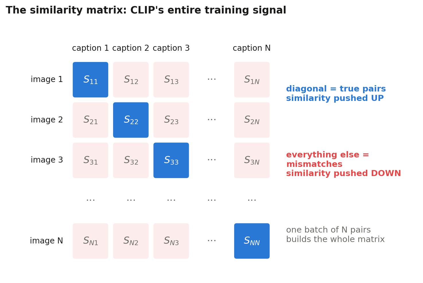
Fig. 1: Every batch builds this matrix. The diagonal holds the true pairs, whose similarity training pushes up; every other cell is a mismatch, pushed down.

Here's the reframe that makes the loss obvious. For image $i$, ask: "which of the $N$ captions in this batch is yours?" That is an $N$-way classification problem, and classification comes with a standard loss: softmax cross-entropy.

Quick refresher, in case it's rusty. A classifier ends in a list of raw scores, one per class; these are called logits. The softmax turns scores into probabilities: exponentiate each score and divide by the sum of all of them, so bigger scores get bigger probabilities and everything sums to 1. Cross-entropy is then the loss: it is $-\log$ of the probability the model assigned to the correct class. If the model assigns the right class probability 1, the loss is 0; if it assigns probability near 0, the loss blows up. Training on this loss does one thing: push the correct class's score up relative to all the others.

Back to our matching problem. The logits for image $i$ are row $i$ of the similarity matrix (how well image $i$ matches each of the $N$ captions), and the correct class is $i$:

$$\mathcal{L}_i^{\text{img}\to\text{txt}} = -\log \frac{e^{S_{ii}/\tau}}{\sum_{j=1}^{N} e^{S_{ij}/\tau}}$$

Do the same for each caption over the images (column-wise), average both directions over the batch, and that's the whole loss. The literature calls it InfoNCE ("information Noise-Contrastive Estimation", though the name matters less than the structure you just derived):

$$\boxed{\;\mathcal{L} = \frac{1}{2N}\sum_{i=1}^{N}\Big[\underbrace{-\log \frac{e^{S_{ii}/\tau}}{\sum_j e^{S_{ij}/\tau}}}_{\text{image picks its caption}} \;+\; \underbrace{-\log \frac{e^{S_{ii}/\tau}}{\sum_j e^{S_{ji}/\tau}}}_{\text{caption picks its image}}\Big]\;}$$

Two details worth unpacking:

The temperature $\tau$. Dot products of unit vectors live in $[-1, 1]$, a pathetically narrow range for logits; the softmax over it is nearly uniform and the gradient is mush. So you divide by a learned temperature $\tau$ (CLIP initializes it to $0.07$ and clamps the resulting logit scale at 100 for stability), which stretches the range to something a softmax can bite into. It's just a logit scale.

The classes are improvised, and that changes everything. Supervised pretraining had 1000 fixed classes chosen by a committee. Here, every batch conjures a brand-new classification problem whose "classes" are whatever $N$ captions it happens to contain, and CLIP trained with $N = 32{,}768$, so each step poses a fresh 32,768-way problem. Same engine as classification, but the label space is no longer a fixed list: anything that can be written can be a class.

supervised:  cross-entropy over 1000 fixed classes      (the label list is the ceiling)
CLIP:        cross-entropy over N improvised classes    (the ceiling is language itself)

In pseudocode, the whole thing:

u = normalize(image_tower(images))          # (N, d)
v = normalize(text_tower(texts))            # (N, d)
S = u @ v.T / tau                           # (N, N) similarity logits

P_img = softmax(S,   axis=1)                # row i: image i's probabilities over the N captions
P_txt = softmax(S.T, axis=1)                # row j: caption j's probabilities over the N images

diag = arange(N)                            # the correct match is the diagonal
loss = (-log(P_img[diag, diag]).mean()      # each image picks its caption
        - log(P_txt[diag, diag]).mean()) / 2  # each caption picks its image

(Real implementations fuse the softmax and the log into a single cross_entropy(S, labels) call, which is numerically stabler; the code above is what that call computes.)

Train that on the 400 million image-text pairs OpenAI scraped from the internet, and you get CLIP.

3.3 The payoff: classification without training

The shared image-text space gives you a party trick that was science fiction in 2020: classification without training. Want a cat-vs-dog classifier? Embed the sentences "a photo of a cat" and "a photo of a dog", embed your image, and see which sentence it's closer to. You just built a classifier out of prose. Any label list, any time, zero training examples. This is "zero-shot" classification, and CLIP's version of it matched a fully supervised ResNet-50 on ImageNet without seeing a single ImageNet label.

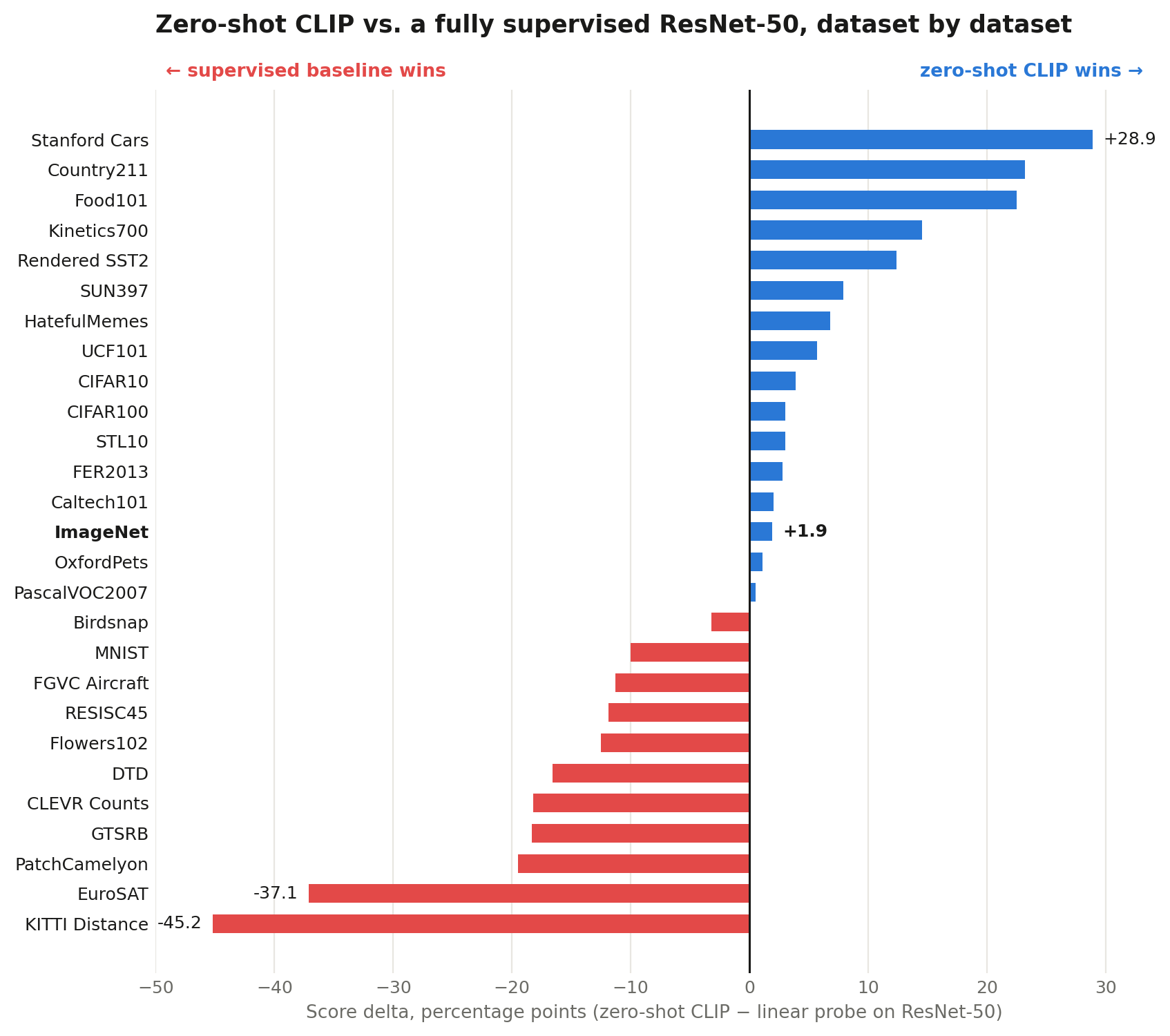
Fig. 2: Zero-shot CLIP (ViT-L/14@336px) against a fully supervised linear classifier trained on ResNet-50 features, across the paper's 27-dataset evaluation suite. Replotted from the data in Radford et al., 2021, Figure 5 and appendix Tables 9 to 11.

The full picture is worth staring at, because the pattern of wins and losses is exactly what the training task predicts. Zero-shot CLIP wins on 16 of the 27 datasets, and it wins where the categories are things people write about: cars, food, scenes, actions. It loses where the task is specialized and nobody captions it: satellite imagery, traffic signs, counting objects, tumor tissue. An embedding knows what its supervision talked about, and alt-text does not talk about lymph node histology.

Retrieval falls out the same way: text-to-image search is literally a dot product now. This is the technology behind every "search your photos by typing" feature you've used.

3.4 The two problems CLIP leaves open

So why isn't CLIP the end of the story? Because it leaves two problems open: one about the infrastructure it takes to train, and a deeper one about what the embedding can and cannot see.

First: the batch is the label space, so the batch must be enormous. Look at the denominator of the softmax: $\sum_j e^{S_{ij}/\tau}$. The "wrong answers" the model learns from are the other captions in the batch. With a batch of 128, discriminating your caption from 127 others is too easy; the task only gets hard, and the embedding only gets sharp, when there are tens of thousands of near-miss distractors. So CLIP-style training runs at batch sizes of 32,768, and because the softmax needs a full row of the similarity matrix, every GPU must gather every other GPU's embeddings each step (an all-gather across the whole cluster) just to normalize. The loss function is dictating your infrastructure.

Second: one vector per image, aligned to what people bother to write. The caption mentions the dog and the sunset. It does not mention that the dog occupies the left third of the frame, or which pixels are dog versus sand. Global, nameable semantics get encoded; spatial, dense structure gets discarded, because the objective never asks for it. Probe a CLIP encoder's patch-level features on segmentation or depth and they're mediocre. Relatedly, later benchmarks that test attribution, relations, and word order (ARO, Winoground) showed these models behave like bags of words: "a dog chasing a cat" and "a cat chasing a dog" land embarrassingly close, because distinguishing them was rarely necessary to win the batch-matching game. (Note this second failure is a property of the matching task itself, not of CLIP's particular loss. That matters because SigLIP, coming next, changes the loss but keeps the task, so it inherits this failure wholesale.)

3.5 SigLIP: swap the softmax for a sigmoid, free the batch

Rewind to the reframe in §3.2: we posed matching as "which caption in the batch is yours?", an $N$-way choice. That framing is why the loss is a softmax, and the softmax is why training needs the giant batch and the all-gather.

SigLIP (Sigmoid Language-Image Pretraining, Google 2023) asks the question differently. Don't make the image pick one caption out of $N$. Instead, for every (image, caption) cell in the $N \times N$ matrix, ask a yes/no question: "is this a real pair?" Diagonal cells: yes. Off-diagonal: no. That's $N^2$ independent binary classifications. Binary classification swaps the softmax for the sigmoid $\sigma$, which squashes a single score into a single probability between 0 and 1, no other classes involved:

$$\mathcal{L} = -\frac{1}{N}\sum_{i=1}^{N}\sum_{j=1}^{N} \log \sigma\big(z_{ij}\,(t\, u_i \cdot v_j + b)\big), \qquad z_{ij} = \begin{cases} +1 & i = j\\ -1 & i \neq j\end{cases}$$

where $t$ is a learned temperature (same job as CLIP's $\tau$) and $b$ is a learned bias. The bias exists because the matrix is wildly imbalanced: each batch has $N$ true pairs and $N^2 - N$ mismatches, so for a random cell the right default answer is "not a pair," overwhelmingly. A freshly initialized model doesn't know that. Its embeddings are random, so every dot product starts near 0, and $\sigma(0) = 0.5$: the model begins by saying "50/50, maybe" for all $N^2$ cells. The first phase of training would then be wasted on one giant, uninformative correction: push every score down until the predictions match the "mostly negatives" reality. Initializing $b = -10$ skips that entirely. With dot products near 0, every cell's starting logit is just $b$, and $\sigma(-10) \approx 5 \times 10^{-5}$, about 1 in 22,000. That is almost exactly the true rate of positives in a 32k batch (1 in 32,768), so the model begins life approximately calibrated, and the gradients can go to the real work from step one: lifting the $N$ true pairs above the crowd. ($t$ starts at 10 for a humbler reason: dot products of unit vectors live in $[-1, 1]$, and multiplying by 10 stretches them into a range the sigmoid can discriminate over. It's the same job CLIP's $\tau$ does for the softmax. Both $t$ and $b$ are ordinary learned parameters after that; these are just their starting values.)

In code, the diff from CLIP is two lines:

S = u @ v.T                                 # (N, N), same as before
z = 2 * eye(N) - 1                          # +1 on diagonal, -1 elsewhere
loss = -log_sigmoid(z * (t * S + b)).mean() # log_sigmoid(x) = log(sigma(x))

The deeper change is in what gets graded together:

CLIP's softmax:   grade each ROW as one N-way contest -> the whole row must
                  be assembled in one place before anything can be scored
SigLIP's sigmoid: grade each CELL as its own yes/no   -> any cell can be
                  scored anywhere, at any time

Why this frees the batch: each cell's loss is now self-contained. There is no denominator summing over the row, so no cell needs to know about any other cell, and the giant $N \times N$ matrix never has to exist in one place. The SigLIP implementation exploits that directly. Each GPU holds its own slice of images and texts, and scores its images against its own texts first. Then every GPU hands its text embeddings to its neighbor, scores its images against the chunk it just received, and repeats until every text chunk has visited every GPU. The loss just accumulates chunk by chunk: the same $N^2$ pairs get scored in the end, but each device only ever holds one small block of the matrix at a time, and the only communication is neighbor-to-neighbor hand-offs instead of an all-gather across the whole cluster.

Image embeddings never move: a pair is scored on whichever device holds the image, so it is enough for the text embeddings alone to travel. A visiting text meeting a foreign image is exactly what we want (those cross pairs are the negatives); each text meets its own image just once, on its home device's diagonal. In pseudocode, per device:

def sigmoid_loss(imgs, txts, matched):
    S = imgs @ txts.T                                 # (b, b) block of similarities
    z = 2 * eye(b) - 1 if matched else -ones(b, b)    # labels: +1 on the diagonal, -1 elsewhere
    return -log_sigmoid(z * (t * S + bias)).sum()     # same loss as above, summed over the block

# D devices; each holds b = N/D of the batch's pairs:
#   my_imgs: embeddings of MY b images   (these never leave this device)
#   my_txts: embeddings of their captions (these will tour the ring)
loss = sigmoid_loss(my_imgs, my_txts, matched=True)     # home block: my b true pairs on its diagonal
chunk = my_txts
for _ in range(D - 1):
    chunk = pass_to_neighbor(chunk)                     # send current chunk right, receive one from the left
    loss += sigmoid_loss(my_imgs, chunk, matched=False) # my images vs someone else's texts: all mismatches
loss /= N                                               # one normalization at the end, as in the equation
# after D-1 hops my images have met all N texts, b x b at a time;
# gradients then average across devices as in any data-parallel setup

And quality no longer depends on a huge batch for normalization: SigLIP matches or beats CLIP at much smaller batches (and the paper's scaling study found that past ~32k, bigger batches stop helping anyway). The result: CLIP-quality models trained with a fraction of the infrastructure pain, which is why so many of today's open VLMs (PaliGemma, Gemma 3, Idefics, MiniCPM-V) run on SigLIP-style encoders.

Notice the shape of this move, because you'll see it again: keep the task, swap the normalization. Nothing about "language supervises vision" changed; one line of loss math did.

3.6 SigLIP 2: one task was never going to be enough

That leaves CLIP's other problem: the features are global-only. The matching task grades one summary vector per image, so nothing in training ever grades where things are. No tweak to the matching loss can change that, because the shortcoming lives in the task, not the loss. So SigLIP 2 (2025) changes the tasks. It trains the same encoder on several tasks at once, chosen so that every property you want in the embedding has a task that grades it:

1. The sigmoid matching task stays. This is what keeps the embedding aligned to text; everything SigLIP could do, SigLIP 2 still does.
2. A captioning task is added. A small decoder transformer is bolted onto the encoder and must generate each image's caption from its features, including phrases that say where objects are. The ground truth costs nothing new: the target caption is the same alt-text already paired with every image for the matching task, and the where-phrases (object names with bounding boxes) are pseudo-labels, drawn automatically by running an existing open-vocabulary detector over the caption's noun phrases. Why does this help? Because matching and generation examine the features differently. Matching is a multiple-choice exam: the features only need enough signal to rank the true caption above the other candidates in the batch, and coarse cues (the right objects, roughly the right scene) usually suffice to win. Generation is a fill-in-every-word exam: the decoder must produce the caption token by token from the image features alone, so every detail the caption mentions has to actually be present in those features. You cannot write "the dog on the left" out of features that never recorded where the dog is.
3. Two self-supervised tasks are added. In the first task, the encoder is shown only a small crop of the image, and from that crop alone it must produce the summary of the whole image. Given a paw and a patch of sand, predict the summary of the whole scene: the only way to succeed is for the features to capture what objects are present and how parts relate to wholes. This setup is called self-distillation. In the second task, half of the image's patches are hidden from the encoder, and it must predict the feature belonging at each hidden position (masked prediction). The first task grades the global summary; the second grades patch vectors individually, at every hidden position. One thing is left hanging on purpose: in both tasks, the target (the whole-image summary, the missing patch features) is produced by a second copy of the encoder that sees the full image. What that second copy is, and why the whole arrangement works, is the story §4 exists to tell. Both tasks come straight from Route B.

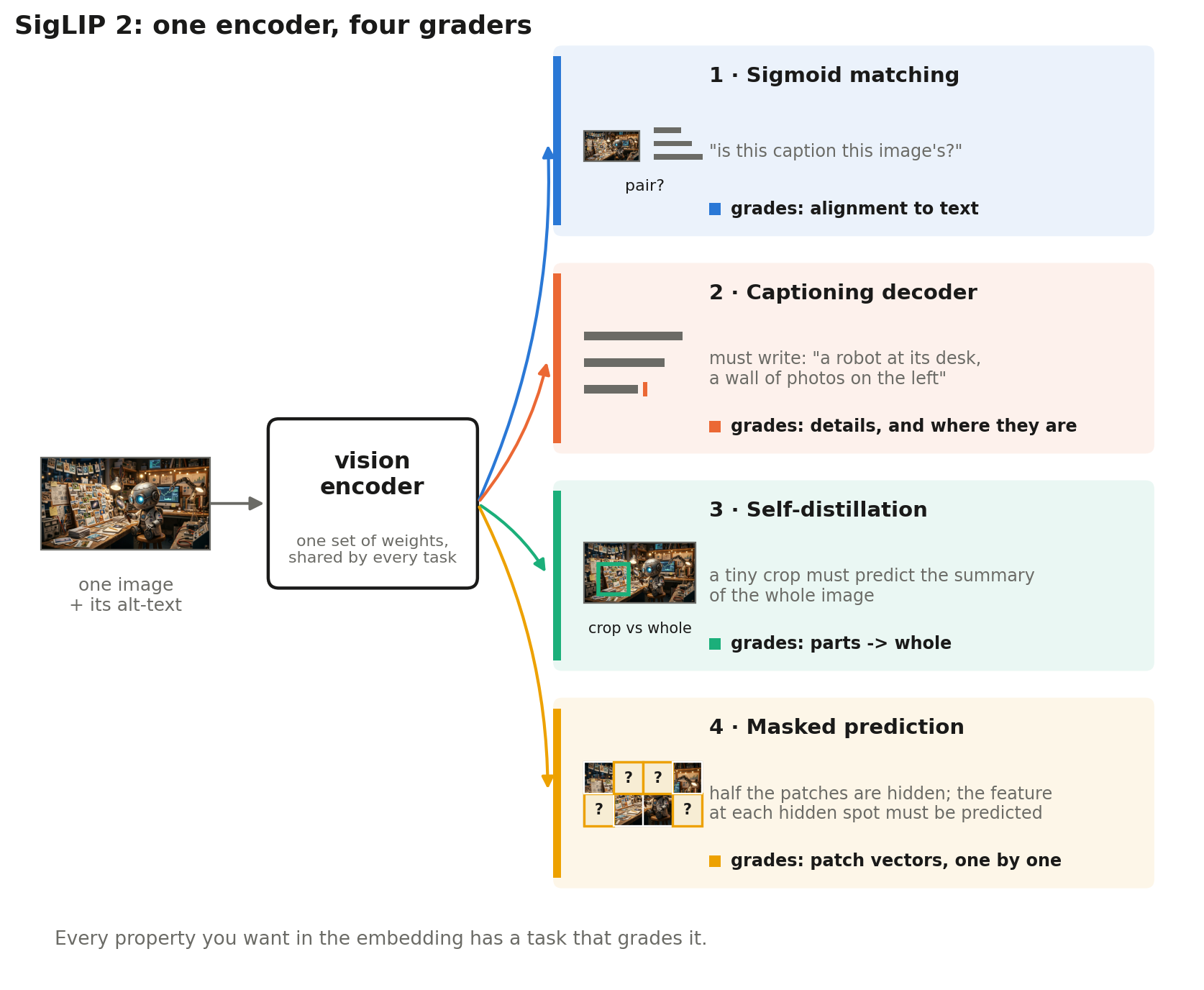
Fig. 3: One shared encoder, four tasks pulling on it at once. Each grades a property of the embedding that the others cannot see.

Two practical upgrades round it out: the training data is multilingual, and the model accepts images at their native resolution and aspect ratio instead of forcing everything into a square (a real difference for documents, screenshots, and anything tall or wide). The result is the text-aligned encoder most new systems reach for today: aligned to language like CLIP, cheap to train like SigLIP, and competent at dense tasks thanks to what it borrowed from Route B.

---

4. Route B: the image supervises itself

4.1 Why bother, when captions are free?

Because language only describes what a human bothered to say. A caption is a lossy, global summary; nobody's alt-text specifies where every edge is, how surfaces are oriented, which patch of pixels belongs to which object, or that these two photos show the same specific dog from different angles. Most of what's in an image has no name. If you want an embedding that captures the image's full structure, especially dense per-patch structure, the supervision has to come from somewhere richer than text.

The only thing richer than a description of the image is the image itself. That's Route B, self-supervised learning: manufacture the training signal out of raw pixels, no text, no labels.

The standard trick for manufacturing it: augmentation. Take our beach photo. Crop it randomly, flip it, jitter the colors, blur it, and you get two mangled views. They came from the same photo, so declare them a positive pair: whatever the encoder outputs for view one should match what it outputs for view two. The encoder is forced to see through the mangling to whatever is stable underneath. "Golden retriever, beach, sunset" survives every crop and color jitter; "pixel (400,300) is orange" does not. Invariance to augmentations, identity of content.

So the objective is: make the embeddings of two views of the same image agree. That sounds complete, but as written it has a fatal flaw. The flaw, and the ways around it, turn out to organize all of self-supervised learning, so it deserves its own section.

4.2 The collapse problem: the central difficulty

Recall the objective we just wrote: two views of the same image should get the same embedding. Now ask: what is the easiest way for the encoder to satisfy it? Notice that the loss only ever rewards agreement. Nothing anywhere rewards telling images apart. So the laziest strategy wins, perfectly: ignore the input and always output one fixed vector. Two views of the beach photo agree (they get the identical vector), two views of every other photo agree just as well, and the loss sits at exactly zero, forever. Every image on Earth lands on the same point, the embedding space collapses to a dot, and the encoder has learned nothing.

Stare at that for a second, because it's not a bug in one method; it's a structural hole in the whole idea. Supervised learning never had this problem: the labels differ across images, so constant output has high loss. CLIP never had it either: the other captions in the batch punish a constant. But the moment your only signal is "agree with yourself," the laziest possible agreement wins. Every self-supervised method is, at its core, an answer to the question: what stops the collapse? The field produced four answers: negatives, asymmetry, regularization, and clustering.

4.3 Answer 1: negatives (SimCLR and MoCo)

The first answer reuses the mechanism CLIP already relies on: pull the two views together and push them away from every other image in the batch. A constant output now fails, because agreeing with your positive means also agreeing with all your negatives, and the repulsion term punishes that.

Mechanically this is InfoNCE again, the exact boxed equation from §3.2, with one substitution: where CLIP pairs an image with its caption, here an image is paired with its other augmented view, and both sides go through the same image encoder. That is all SimCLR (a Simple framework for Contrastive Learning of visual Representations) is: CLIP with the text tower thrown away and the image tower used for both sides.

And because it's the same loss, it inherits the same batch-size problem from §3.4: the negatives come from the batch, so the batch must hold thousands of them for the task to be hard. SimCLR answered by simply paying the cost: it ran at batch 4096.

MoCo (Momentum Contrast) answered by questioning the premise. A negative is just an embedding you push away from, and nothing says it has to come from the current batch. So MoCo keeps a queue of embeddings from the last several batches and uses those as the negatives: the model compares against tens of thousands of them while the actual batch stays small. One catch: the queued embeddings were produced by slightly older versions of the encoder, so MoCo computes them with a slowly updated moving-average copy of the network to keep them consistent. That copy is the "momentum" in the name. Remember it, because the same idea is about to take center stage.

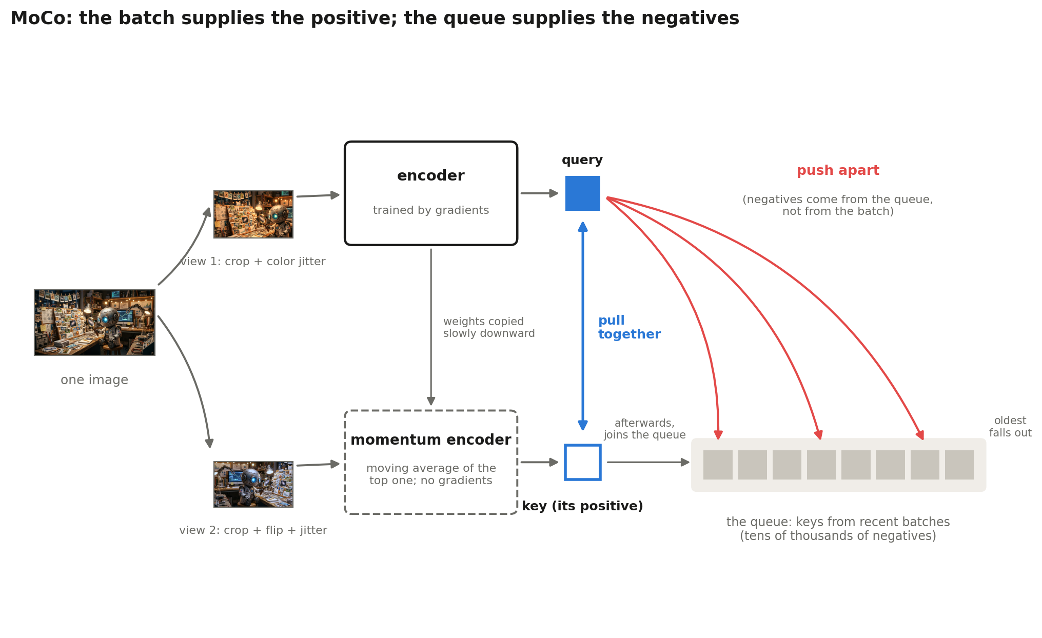
Fig. 4: MoCo's split of labor: the current batch supplies each query's positive; the queue of keys from recent batches supplies the negatives. The momentum encoder, a slowly updated moving average of the trained encoder, keeps the queued keys consistent.

Whichever way the negatives are supplied, one problem remains, and it belongs to the whole family: the loss actively pushes apart two different photos of golden retrievers on beaches, because they happen to be "negatives." The repulsion that prevents collapse is also fighting the semantics you want.

4.4 Answer 2: no negatives, an unequal fight (BYOL and DINO)

The second answer is stranger, and it turned out to be the winner. Keep the objective "two views of the same image should agree" and delete the negatives. But change who is agreeing with whom. In the broken setup, one network compares its own two outputs, so it can satisfy the objective by outputting anything it likes, as long as it always outputs the same thing. Instead, send the two views through two different versions of the network, where only one of them is being trained, and it must match the output of the other: a target its own gradients cannot touch. Why that blocks the shortcut to collapse will become clear in a moment. First, the two versions:

• The student is the network being trained. It gets the gradients, as usual.
• The teacher is a second copy of the same architecture. It is never trained. Instead, after every step, its weights drift a small fraction of the way toward the student's current weights, making it a slow-moving average of the student's own past (an exponential moving average, EMA). This is exactly MoCo's momentum copy, promoted from a supporting role to the main mechanism.

The training rule: looking at view 1, the student must predict what the teacher outputs for view 2. BYOL (Bootstrap Your Own Latent, DeepMind 2020) was the first to show this works with no negatives at all. DINO (self-distillation with no labels, Meta 2021) is the version that conquered ViTs, and the one worth understanding in detail.

First, a gap to fill: an encoder outputs an embedding vector, so what does "predict what the teacher outputs" actually mean? DINO adds a small projection head that maps the embedding to scores over $K$ slots (DINO uses $K = 65{,}536$). Nobody labels the slots. They are pseudo-categories the model is free to invent, and over training each slot ends up firing for some recurring visual pattern: one slot for furry textures, say, another for sunsets, another for wheels. A softmax turns the scores into a probability distribution over the slots, and the loss is the familiar cross-entropy: the student's distribution for its view must match the teacher's distribution for the other view. Mechanically this is classification yet again, except the "correct answers" come from the teacher instead of from human labels. Training one model to match another model's output distribution is called distillation, hence DINO's full name; the twist is that there is no pretrained teacher. The teacher is the student's own past, averaged. The model distills itself.

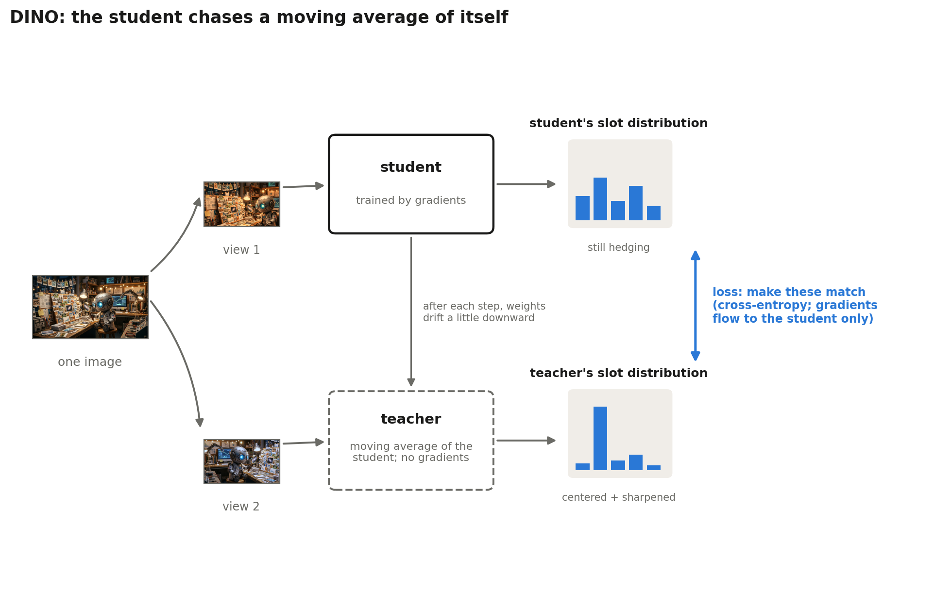
Fig. 5: One DINO training step. The student, from its view, must reproduce the slot distribution the teacher produced from the other view. The teacher is never trained; after every step its weights only drift a little toward the student's.

Now, why doesn't this collapse? The asymmetry closes the fast lane: the teacher takes no gradients, so the optimizer cannot drag the target down into a constant the way it could when both sides were the same trained network. But a slow drift into collapse is still possible, and for an output that is a distribution over slots, collapse has exactly two flavors:

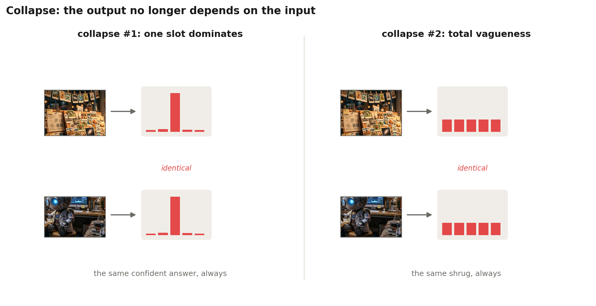
Fig. 6: The two ways a distribution over slots goes dead. Left: one slot wins for every image, so the output is the same confident answer no matter what comes in. Right: every slot gets the same score $1/K$ for every image, the same shrug no matter what comes in. Different failures, same symptom: the output stopped depending on the input.

Both are dead for the same reason: the output no longer depends on the input. DINO blocks each with a correction applied to the teacher's scores, and the two corrections deliberately pull in opposite directions:

• Centering blocks collapse #1. Keep a running average of the teacher's scores over recent images, and subtract it. A slot that fires for every image builds up a large average, so the subtraction cancels exactly the image-independent part of each score. Whatever survives centering is, by construction, the part that differs from image to image.
• Sharpening blocks collapse #2. Divide the scores by a temperature below 1 before the softmax, which exaggerates whichever slots are ahead for this particular image. The teacher is forced to commit to an opinion instead of shrugging.

Centering alone herds every output toward the uniform shrug; sharpening alone lets one slot run away with everything. Balanced against each other, they leave exactly one stable option: outputs that are confident and different from image to image. Which is another way of saying: informative.

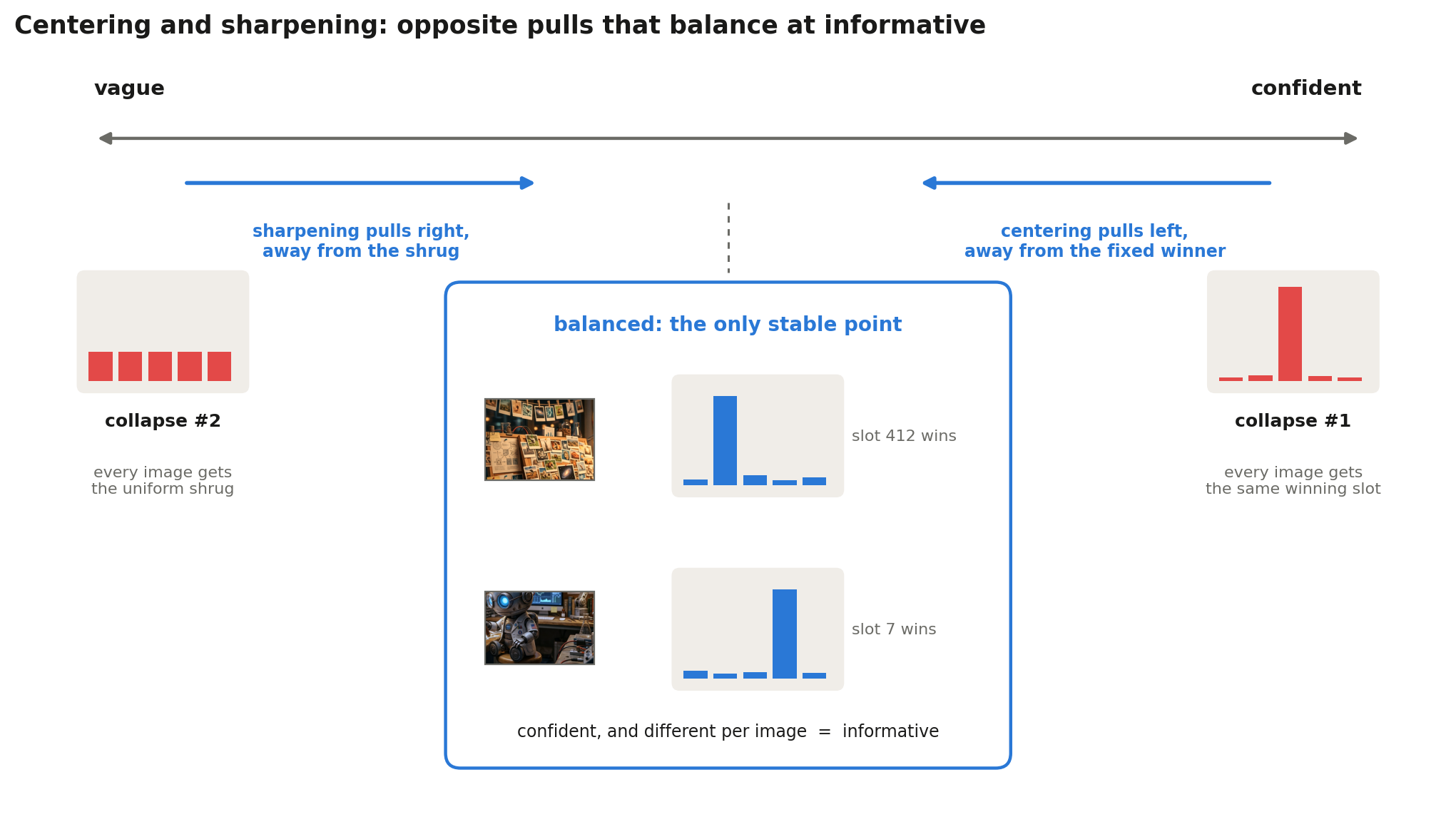
Fig. 7: The tug-of-war. Each collapse sits at one end of the vague-to-confident axis, and each correction pulls away from one of them: sharpening away from the shrug, centering away from the fixed winner. Where they balance, the teacher must stay confident while no slot dominates across images, and the only way to do both is for different images to win different slots.

Note: It's fair to be suspicious of the whole arrangement. Why would a model chasing an average of its own past outputs learn anything, rather than chase its tail? The honest intuition: an EMA of many past students behaves like an ensemble of them, and ensembles are reliably a bit better than any single member. So the target is always slightly ahead of the student, the student improves to catch it, which improves the teacher, which moves the target ahead again. It shouldn't work as well as it does, and the theory still trails the practice. But it works.

The whole training loop, with one detail the diagram above simplified away: the prediction rule works in either direction, so both networks embed both views and the loss adds the two crossed pairings (student on view 2 chasing teacher on view 1, and the reverse). Same rule, applied twice, two training signals from one pair of views:

for x in loader:
    v1, v2 = augment(x), augment(x)               # two views of the same image

    r1, r2 = teacher(v1), teacher(v2)             # teacher's raw slot scores, no gradients

    t1 = softmax((r1 - center) / tau_t)           # teacher's slot distributions:
    t2 = softmax((r2 - center) / tau_t)           #   centered, then sharpened (tau_t < tau_s)

    s1 = softmax(student(v1) / tau_s)             # student's slot distributions
    s2 = softmax(student(v2) / tau_s)

    loss = H(t1, s2) / 2 + H(t2, s1) / 2          # cross-entropy, views crossed: student on v2
    loss.backward(); opt.step()                   #   chases teacher on v1, and vice versa

    teacher_w = m * teacher_w + (1 - m) * student_w         # teacher drifts toward student
    center    = c * center + (1 - c) * cat(r1, r2).mean(0)  # running mean of RAW teacher scores

One more ingredient matters: multi-crop. The teacher only ever sees large crops that cover most of the image; the student also receives several tiny crops and must still match the teacher from them. From a patch of sand and one paw, predict the summary of the whole scene. This local-to-global prediction is a big part of why DINO's features come to understand objects and context rather than just textures. It is also the exact task SigLIP 2 later imported as its "self-distillation" objective (§3.6); this is where that idea lives natively.

Then came the result that put DINO on the map. In a ViT, the CLS token's attention weights record which patches it is reading from when it builds its summary. Plot those weights for a trained DINO model as a heatmap over the image, and the heatmap traces the dog against the beach cleanly: with no labels and no segmentation supervision, the model has learned to segment objects. Ask CLIP's encoder where the dog is and it shrugs; it was never asked. DINO was never asked either, but the task of matching views across aggressive crops apparently requires knowing what's foreground. This is the moment it became clear Route B wasn't a budget substitute for labels; it was learning things labels don't teach.

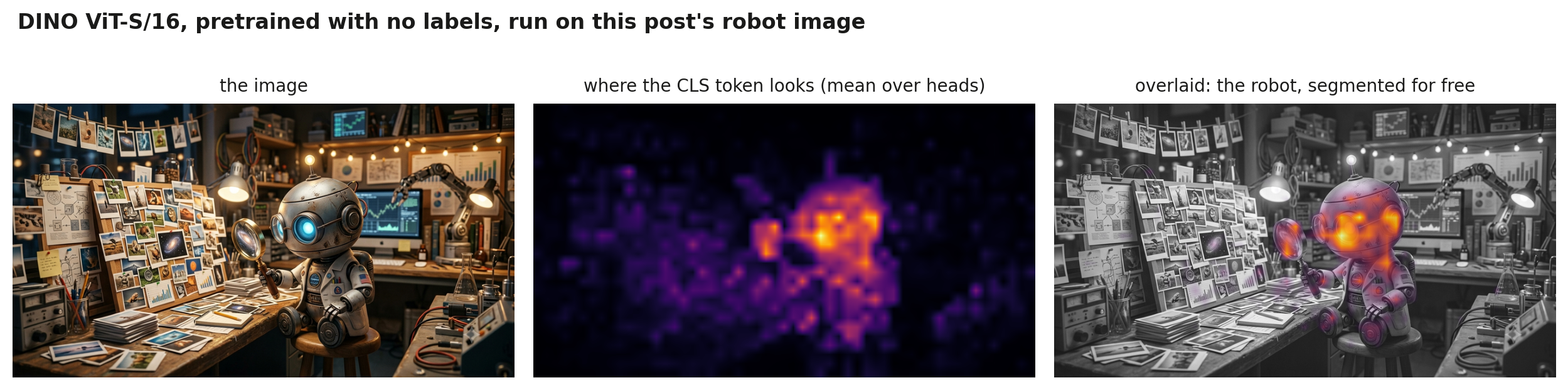
Fig. 8: A pretrained DINO ViT-S/16 run on the robot image from the top of this post, using the visualization from Caron et al., 2021. Middle: the final layer's CLS-token attention over patches, averaged across heads. Right: the same map overlaid on the image. Nothing ever told the model the robot is the subject; separating foreground from clutter fell out of training.

4.5 The answers nobody scaled: regularizers and clusters

The field produced two more answers to collapse. Neither was scaled up the way self-distillation was, so we will not go into detail here: each gets a sketch of its core idea, and the linked papers are the place to go for the full mechanics. The sketches are still worth reading, because pieces of these ideas survive inside the models that won (§4.7).

Answer 3: outlaw collapse directly. Barlow Twins and VICReg (Variance-Invariance-Covariance Regularization) use no negatives and no teacher. They pull the two views together and attack collapse with regularization. VICReg is the explicit version: a variance term forces every embedding dimension to keep high variance across the batch (a collapsed embedding has zero variance, which is now simply illegal), and a covariance term forces different dimensions to stay decorrelated, so the embedding can't hide redundant copies of one feature. Barlow Twins gets the same effect indirectly: batch-normalize the embeddings, then push the cross-correlation matrix between the two views toward the identity; the diagonal enforces invariance, the off-diagonal enforces decorrelation, and a collapsed embedding can't satisfy either. Note the difference in strategy: BYOL and DINO prevent collapse through the training arrangement (the teacher-student asymmetry), while these methods put it in the loss itself, adding terms that any collapsed embedding scores badly on. (SimSiam is the strange little datapoint at the minimal end: no negatives, no EMA, no regularizer. Just a predictor head on one branch and a stop-gradient on the other, and it still doesn't collapse. Why, exactly, is still not fully settled, which tells you how empirical this corner of the field remains.)

Answer 4: cluster, but keep the clusters balanced. DeepCluster and SwAV (Swapping Assignments between Views) assign images to learned clusters and require two views of the same image to land in the same cluster, with the assignments explicitly balanced (SwAV uses the Sinkhorn-Knopp algorithm for this) so that everything can't pile into one mega-cluster. Balanced clusters are themselves an anti-collapse constraint.

At scale, the self-distillation family won the benchmarks. But look inside DINOv2 (§4.7) and you'll find the other answers absorbed rather than defeated: its teacher normalization is SwAV's Sinkhorn-Knopp, swapped in for DINO's original centering, and its KoLeo term (named for the Kozachenko-Leonenko entropy estimator it's built on) is a spread-the-features regularizer in exactly the VICReg spirit.

4.6 The missing piece: supervision per patch, not per image

Everything so far (CLIP's matching, SimCLR's contrast, DINO's distillation) grades the encoder on one global vector per image. But a ViT naturally produces a vector per patch: a 224×224 image cut into 14×14-pixel patches is a 16×16 grid, so 256 patch vectors. For dense work (segmentation, depth, correspondence), those patch vectors are the product. Nothing yet has trained them directly.

The masked-modeling family fixes that with the oldest self-supervision trick in the book, the one BERT (Bidirectional Encoder Representations from Transformers) built language pretraining on: hide part of the input, predict it from the rest. MAE (Masked Autoencoders, 2021) masks 75% of patches and reconstructs the pixels. It works, but pixel reconstruction wastes capacity on texture and noise that no downstream task cares about. The refinement, iBOT (image BERT pretraining with Online Tokenizer), is to reconstruct masked patches not in pixel space but in the teacher's latent space: the student sees the masked image and must predict, for each hidden patch, the distribution the EMA teacher assigned to it when the teacher saw the full image. You should recognize this instantly: it's the DINO loss, applied per patch. Same teacher, same centering-and-sharpening, same self-distillation, just asked 256 times per image instead of once.

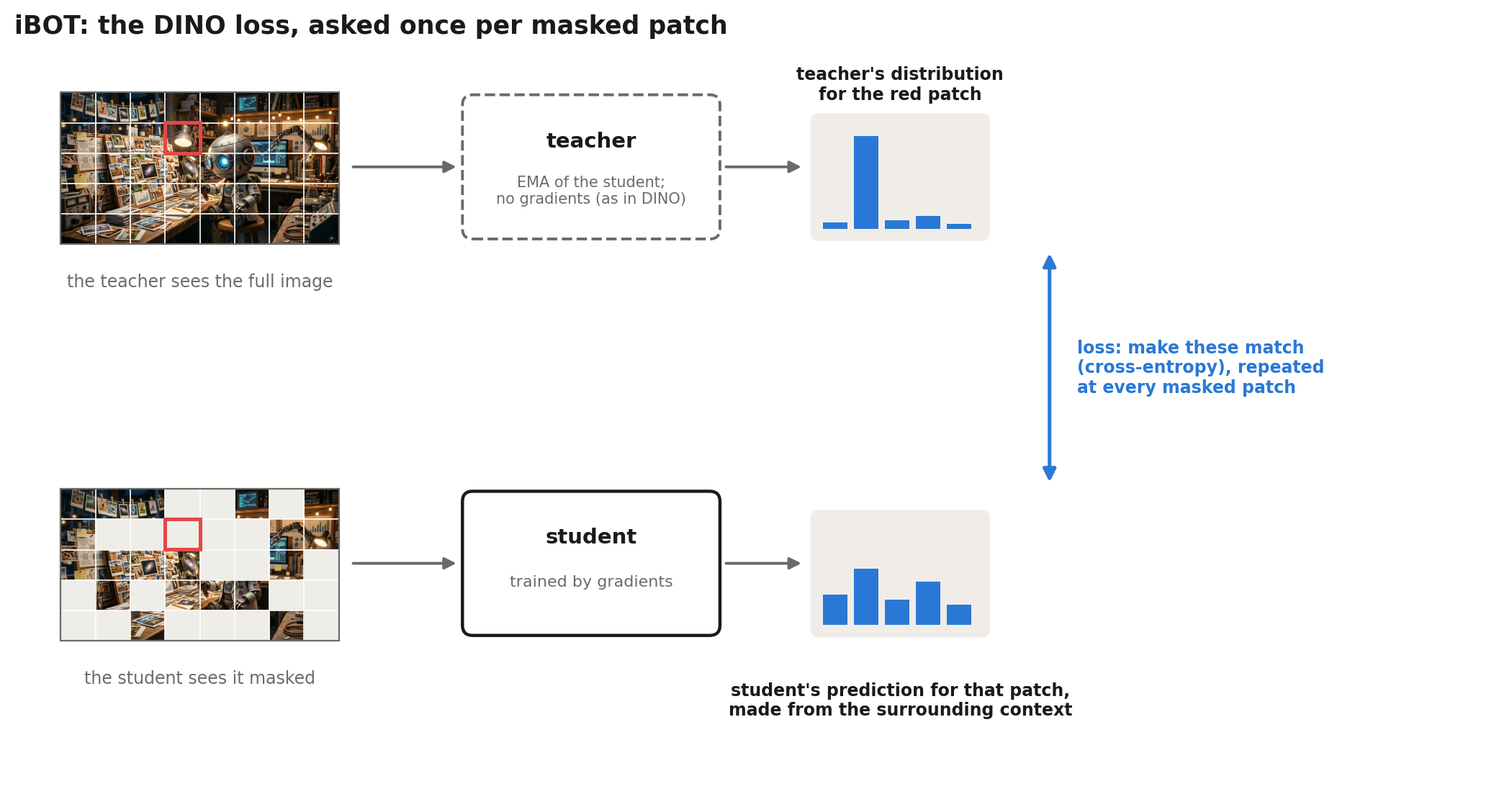
Fig. 9: One iBOT training step, shown for a single masked patch (outlined in red). The teacher sees the full image and produces a slot distribution for every patch; the student sees the masked image and must predict, from the surrounding context alone, the distribution the teacher assigned to each patch it cannot see. The same matching loss fires at every masked patch, 100+ times per image.

Now every patch vector gets its own gradient, and dense features get trained on purpose rather than by accident. (And that closes the other loop from §3.6: this is the "masked prediction" task SigLIP 2 imported. Both of its borrowed objectives are now accounted for.)

4.7 DINOv2: the recipe industrialized

DINOv2 (Meta 2023) introduced no new core idea. Its contribution is engineering: it combined the pieces built up over the previous sections, tuned them, and scaled them into a backbone other teams could build on. Three decisions did the work.

The first decision is the loss. DINOv2 trains DINO's image-level self-distillation and iBOT's patch-level masked distillation side by side, so one model learns global semantics and dense features at the same time. The anti-collapse machinery is the upgraded version you already met in §4.5: SwAV's Sinkhorn-Knopp normalization replaces DINO's centering, and the KoLeo regularizer nudges embeddings to spread uniformly over the sphere.

The second decision is data curation, and it matters more than it sounds. Raw web images are full of duplicates and junk, and a self-supervised model, having no labels to steer it, learns whatever distribution it is fed. So DINOv2 builds its own: start from roughly 1.2 billion uncurated web images, deduplicate, then use an existing embedding model to retrieve the images most similar to a curated seed corpus. The result is LVD-142M, 142 million images with the diversity of the web but the distribution of a clean dataset. Notice the loop: embeddings curate the data that trains better embeddings.

The third decision is to scale first and distill after. Train one big ViT-g (about 1.1 billion parameters), then distill it into small, base, and large students, so the sizes people actually deploy inherit the giant's quality.

The payoff was a genuine phase change: a frozen DINOv2 backbone (no fine-tuning, just linear probes) matched or beat supervised and CLIP-style features on classification, and dominated dense tasks (depth, segmentation, correspondence) where CLIP-family encoders were weakest. The pitch became: stop fine-tuning backbones; embed once, probe cheaply.

4.8 DINOv3: scale, and the problem it exposed

DINOv3 (Meta 2025) pushes the recipe further: a 7-billion-parameter ViT trained on about 1.7 billion curated images. But the more instructive part of the paper is the failure mode the team hit on the way. Train that large and that long, and global metrics keep climbing while the dense features quietly degrade: patch embeddings that were crisp and local earlier in training turn noisy and smeared, and segmentation probes get worse as training continues. What is happening: the model is slowly reallocating its patch capacity toward what the image-level losses reward, which is global abstraction, and away from local fidelity, which nothing in the loss is grading anymore.

The fix is gram anchoring. Start from what dense tasks actually consume: not any particular feature values, but the relational structure between patches, which patches are similar to which. That structure is captured by the Gram matrix, the patch-by-patch similarity table ("these 40 patches are all dog, those 200 are all sand"). Gram anchoring takes a snapshot of an earlier checkpoint, from before the degradation set in, and adds a loss that keeps the current model's Gram matrix close to the snapshot's. The feature values stay free to keep improving under the global losses; only the patch-level similarity structure is pinned in place. With this term added, global quality keeps climbing while dense quality stops decaying.

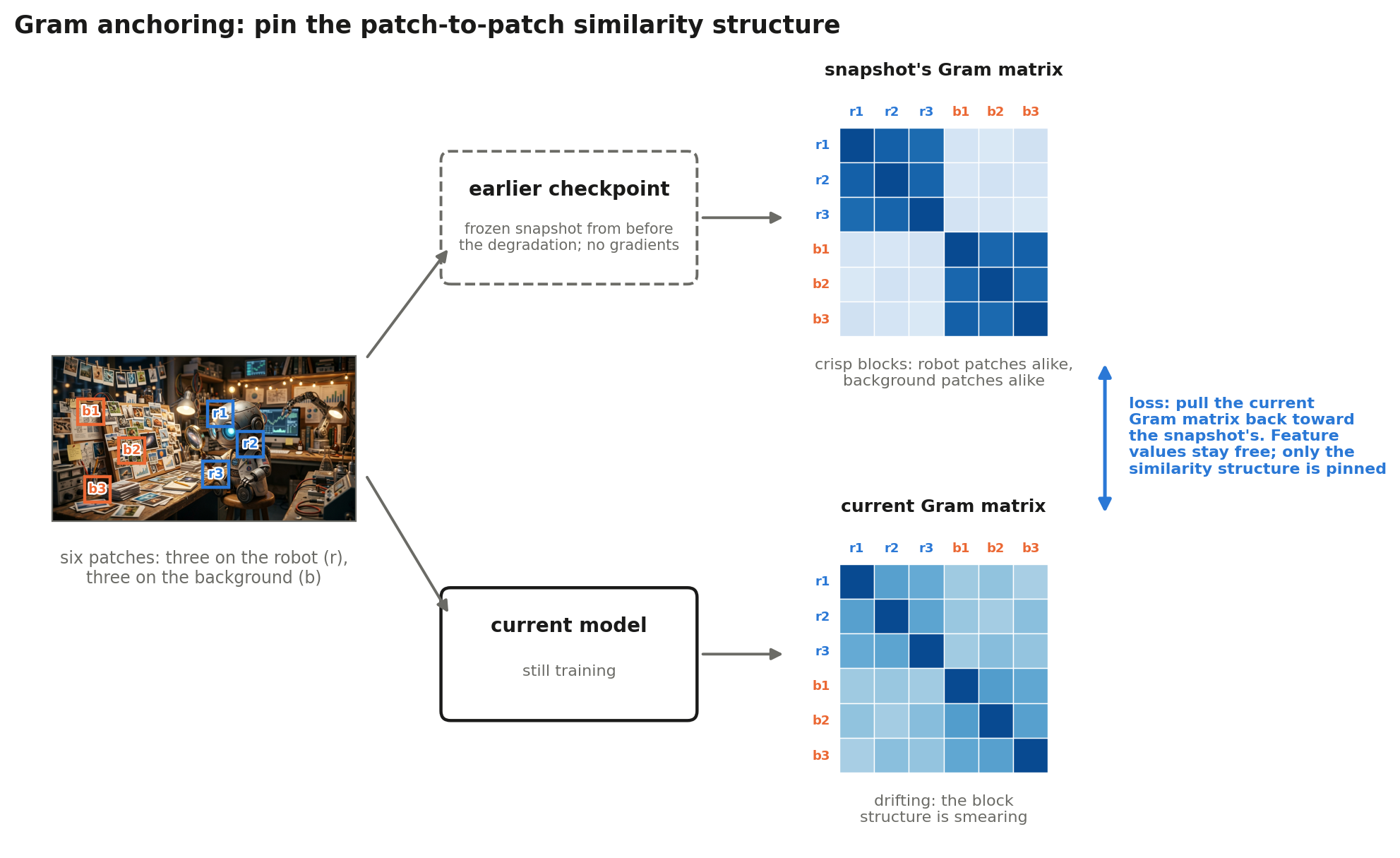
Fig. 10: Gram anchoring, on six patches of our image: three from the robot (r1 to r3), three from the background (b1 to b3). In the earlier checkpoint's Gram matrix the block structure is crisp: robot patches are similar to each other, background patches to each other, and the two groups are distinct. In the still-training model that structure is smearing. The anchoring loss pulls the current Gram matrix back toward the snapshot's, while the feature values themselves stay free to improve.

Note: how is the anchor checkpoint chosen? The degradation is measurable during training: a segmentation probe on the patch features peaks around 200k iterations and then declines, even as classification keeps climbing. Any checkpoint from before that peak works as the anchor; the paper finds 100k and 200k equally good. The anchor also doesn't stay ancient: once the anchoring loss is active the structure stops dissolving, so the Gram teacher is refreshed every 10k iterations with the current model.

Ship the 7B model, distill a family of deployable sizes from it (plus a text-aligned variant, so text-to-image retrieval works too), and you have the current endpoint of Route B: one frozen backbone whose features beat specialized, fine-tuned pipelines on dense benchmarks, detection and segmentation among them. That is further than supervised pretraining ever got.

---

5. The map: the whole zoo on one axis

Step back and the whole zoo collapses into one family tree:

supervised classification            "similar = same label"
 │    labels are expensive, and the label list caps the semantics
 │
 ├── Route A: text as supervisor     "similar = same description"
 │    ├─ CLIP      match images to captions; softmax over the batch; zero-shot everything
 │    ├─ SigLIP    same task, per-pair sigmoid; the batch is freed
 │    └─ SigLIP 2  + captioning + patch-level objectives; dense features arrive
 │
 └── Route B: image as supervisor    "similar = same image, viewed differently"
      ├─ SimCLR/MoCo     agree across augmented views; negatives hold off collapse
      ├─ BYOL -> DINO    no negatives; EMA teacher, centering vs. sharpening
      ├─ Barlow/VICReg   collapse outlawed by regularizer       \  absorbed into
      ├─ SwAV            collapse outlawed by balanced clusters /  DINOv2's recipe
      ├─ + iBOT          the same self-distillation, applied per patch
      ├─ DINOv2          DINO + iBOT + curated data + scale, distilled to every size
      └─ DINOv3          7B scale, gram anchoring keeps the dense features crisp

And the two routes land at two genuinely different products, separated by one axis: aligned to language versus faithful to the image. CLIP-family embeddings live in a space shared with text: you can query the space with words, but it only encodes what text tends to mention. DINO-family embeddings know nothing of words, but they encode the image's actual structure, down to the patch. Neither dominates; they answered different questions. That difference translates directly into a usage guide:

You want	Reach for	Why
Zero-shot classification, text→image search	SigLIP 2 (or any CLIP descendant)	You need the text door into the space
Vision encoder for a VLM	SigLIP 2, increasingly with DINOv2/v3 features mixed in	The LLM speaks language; a text-aligned space is half-translated already
Segmentation, depth, correspondence, tracking (frozen backbone + probe)	DINOv3 / DINOv2	Patch features were trained on purpose, not as a side effect
Image→image search ("more like this one")	DINOv2/v3	No caption bottleneck; visual similarity, not describable similarity
Few-shot classifier (linear probe on 50 examples)	DINOv2/v3 or SigLIP 2	Both spaces are linearly clean; try both, it's ten minutes

The VLM row deserves a closer look: multimodal LLMs overwhelmingly use CLIP-family encoders, which is exactly why they inherit CLIP-family blind spots. Ask one to count objects or judge spatial layout and it often fails, because those are properties captions rarely spell out. A growing line of work (Eyes Wide Shut, Cambrian-1) addresses this by feeding the LLM DINO features alongside the CLIP-style ones, so the two routes end up converging inside the same model.

A field guide to other names you'll meet, each placeable on the map:

• OpenCLIP: an open reproduction of CLIP on open data; same math.
• ALIGN (A Large-scale ImaGe and Noisy-text embedding): Google's CLIP counterpart, the same loss on 1.8B noisier pairs; proof that scale can make up for noisy alt-text.
• CoCa: contrastive matching and caption generation in one model; the idea SigLIP 2's decoder descends from.
• EVA-CLIP: CLIP warm-started from masked-image-modeling weights; Route B boosting Route A.
• I-JEPA (Image-based Joint-Embedding Predictive Architecture): masked prediction in latent space like iBOT, but with no augmentations at all; predict hidden regions from context and position alone.
• AIMv2 (Autoregressive Image Models, v2): Route A rebuilt on autoregressive prediction instead of contrast; generate the caption (and pixels), GPT-style.
• Perception Encoder: Meta's 2025 bet that a single well-tuned contrastive model, probed at the right internal layers, can serve global and dense tasks at once.
• RADIO (Reduce All Domains Into One) and Theia: "agglomerative" backbones that distill several teachers into one student (CLIP + DINOv2 + SAM, the Segment Anything Model, in RADIO's case); the convergence of the routes, done by direct distillation.
• E5-V and VLM2Vec: skip the standalone encoder entirely; prompt a full multimodal LLM and read the embedding out of its hidden state. A genuinely new answer to who defines similar: the LLM does.
• Matryoshka embeddings: a training trick, not a model; train so every prefix of the vector is a usable embedding, letting you truncate to your storage budget.

When the next new checkpoint appears, ask two questions of it (who defines "similar"? and what stops the collapse?) and you will know where on this map it lives.

And the borders of the map. This post covered general-purpose semantic encoders; three neighboring territories were deliberately left out. Supervised metric learning (FaceNet, ArcFace): when you know exactly which distinction you care about ("similar = same person's face", "similar = same product"), you train the margin between identities directly, and this is still how face recognition and product search are built. Generative latents (VAE codes, VQGAN tokens, diffusion features): representations optimized for reconstruction, a different contract than similarity, though diffusion features turn out to work surprisingly well at dense correspondence. Video (V-JEPA and friends): the same story plus time, and a post of its own.

---

6. The one-paragraph version

An embedding model is never trained directly: you pick a pretext task and the embedding is the residue, so the entire zoo is just a list of answers to "who defines what similar means?" Supervised pretraining says the label list, and is capped by it. CLIP says language: match images to captions with a softmax over the batch (classification with improvised classes), buying zero-shot everything at the cost of giant batches and text-shaped blind spots; SigLIP swaps the softmax for independent sigmoids and frees the batch; SigLIP 2 bolts on generative and patch-level tasks to cover the blind spots. The DINO line says the image itself: make two augmented views agree without collapsing to a constant, first via negatives (SimCLR, InfoNCE again), then via self-distillation against an EMA of your own past weights (DINO), extended to per-patch targets (iBOT), industrialized with curated data and distillation (DINOv2), and stabilized at 7B scale with gram anchoring (DINOv3). Text-aligned when you need to talk to the space; self-supervised when you need the space to be true to the pixels. And the frontier is busy combining the two, feeding both kinds of features to VLMs and distilling both kinds of teacher into single backbones.

supervised   ->  similar = same label                (capped by the label list)
CLIP/SigLIP  ->  similar = same description          (speaks language; global, nameable things)
DINO family  ->  similar = same image, seen twice    (speechless; dense, spatial, faithful)